4 Assembling a Data Visualization Application
This chapter begins a set of tutorials that introduce various aspects of AVS/Express. This chapter introduces procedures and techniques for building a data visualization application using existing AVS/Express application components. The application that you will create reads an AVS field data file, creates an isosurface using the field data, and renders the isosurface in a full-featured data viewer.
As you complete the tutorial, you:
- Start AVS/Express
- Instance Objects in the Network Editor
- Connect Objects
- Save Your Application
- Execute Your Application
The remaining chapters in this book build upon the application that you create in this chapter to introduce other techniques such as: modifying an existing application; creating components; integrating code; creating a user interface, and compiling an application.
The procedure below assumes that:
- AVS/Express is installed
- AVS/Express is licensed
- All platform-appropriate environment variables are set (PATH, MACHINE, DISPLAY, LD_LIBRARY_PATH, SHLIB_PATH, and XP_PATH).
If these assumptions are not met, refer to the Installing AVS/Express book and follow the appropriate instructions before continuing.
- Visualization Edition users type:
- Developer Edition users type:
- Note: Do not start AVS/Express in the background. You start AVS/Express in the foreground because AVS/Express' V Command Processor (VCP) uses the shell window.
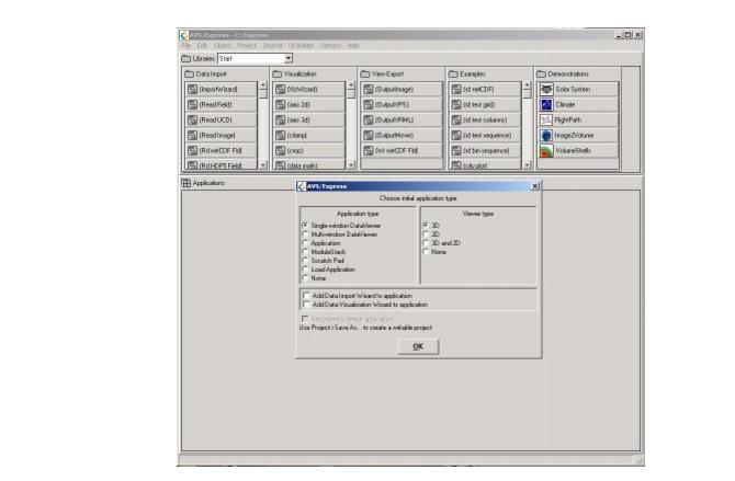
24. The V Command Processor (VCP) appears.Then the Network Editor window appears along with a dialog box that allows you to choose an application framework:
- You can use the Application and Viewer type options to define the type of display, or viewer, that will be used in your application. You will work with other types of applications later in this book.
- The defaults specify that the viewer window and a set of DataViewer editors will be displayed in a single window and that images will be viewable in three dimensions. You can choose an application that displays the viewer and DataViewer panels in separate windows, or choose application frameworks that do not include the DataViewer at all. In this dialog box, you can also add a Data Import Wizard and/or a Data Visualization Wizard to help you with your application.
- Two things happen once you have made your selection:
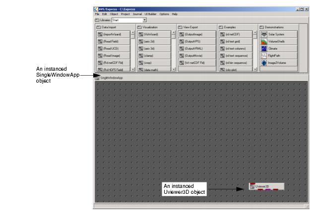
The Network Editor is your primary development environment for creating objects and applications. The title bar reads "AVS/Express," followed by the name of the start-up project directory. You will learn more about projects later.
The SingleWindowApp workspace is an AVS/Express object that functions as the parent object for your application. It automatically includes the Uviewer3D object in its workspace.
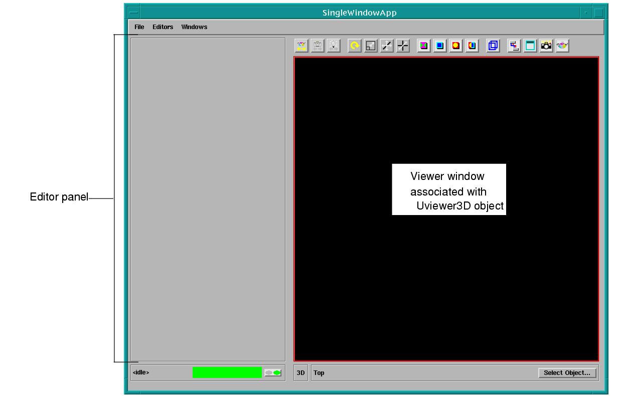
The DataViewer window has two distinct areas. The left side of the window is used to display DataViewer editor panels and module object controls. The area on the right is the viewer area associated with the Uviewer3D object; it is where the rendered data is displayed.
You use the DataViewer editor panels to control rendering and interaction in the viewer window. The module controls are interfaces to the module objects. The controls are automatically added to the editor panel when you add the objects to the application workspace. You will learn more about the editor panels when you work with the Read_Field object later in this chapter.
On UNIX systems, the VCP appears in the shell window where you started AVS/Express. On Windows systems, a new command shell appears containing the VCP. The VCP prompt is shown below:
The V Command Processor (VCP) is an interface with which you can also develop and debug AVS/Express applications. However, rather than the graphical interface provided the Network Editor, the VCP is a textual interface. In the VCP, you perform operations in AVS/Express by entering V command language commands. The V command language (also called V code or V) is a schema definition language with which AVS/Express defines objects and applications.
Through the VCP, you can write V code to perform tasks such as the following:
- Create objects and assign values to them
- Cause objects to persist
- Create networks by connecting objects
- Save networks
The VCP processes your V code, instructing AVS/Express to perform the specified tasks. Note that the VCP is not a compiler; V is an interpreted language rather than a compiled one.
AVS/Express use V code to store the definitions of objects (whether created in the Network Editor or the VCP) in files called V files. Typically, these objects are stored in text V files, whose names, by convention, have the extension .v; for example, my_object.v. However, you can also store object definitions in binary V files, which load into AVS/Express faster. By convention, binary V files have the extension .vo; for example, my_object.vo.
This Getting Started guide uses the Network Editor almost exclusively. For more information about how to use the V command language, see Chapter 8, "V and the V Command Processor" in the book Using AVS/Express.
You begin building an application by selecting the AVS/Express objects that are needed to perform the task at hand. You select objects in the Libraries section of the Network Editor and include them in the application by dragging the objects into the application workspace. This process is called instancing. When you instance an object, the AVS/Express Object Manager executes the functionality associated with that object.
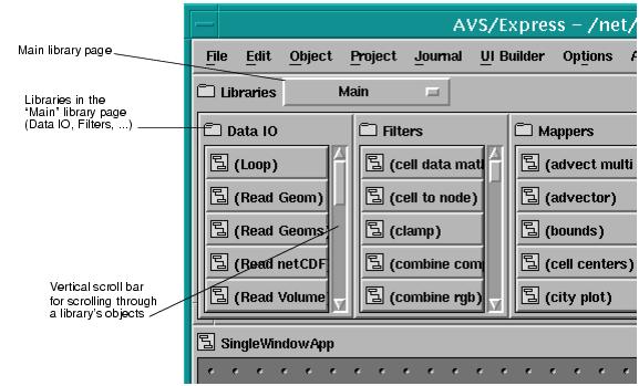
To help you navigate through the AVS/Express objects, they are organized into libraries and sublibraries. The listing of the contents of a particular library in the Network Editor is called a library page. When you start AVS/Express, the Main library page is displayed. It contains high-level objects that enable you to readily construct visualization applications. As on other library pages, the objects in the Main library are catagorized and then oranized into sublibraries. In the case of the Main library page, these sublibraries include: Data IO, Filters, Mappers, Geometries, and so on. The folder icon is used to represent a library or sublibrary.
The objects, as they reside in the libraries, are called templates. It is from these templates that you create executable instances of an object.
Practice viewing the libraries and objects on the Main library page using the procedure below.
- drag the sublibrary's vertical scroll bar to view the library's objects
- -or-
- click on the arrows at the top and bottom of the scroll bar
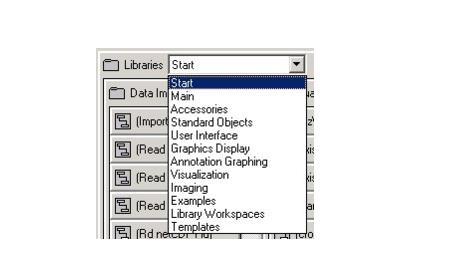
When you start AVS/Express, the Start library page is displayed in the Network Editor. You can display other library pages by using the Libraries drop down menu.
Take a quick tour of some of the other library pages. Start with Standard Objects.
a. To select the an item from this type of menu, move the mouse over the drop down menu, and then press and hold the left mouse button.
- The drop-down menu appears, and it lists the libraries installed in AVS/Express.
b. While still pressing the mouse button, move the pointer to the desired menu item and then release the mouse button. In this case, select Standard Objects.
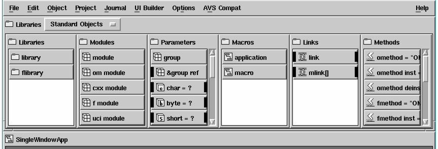
- The Network Editor displays the Standard Objects library page.
The Standard Objects library contains AVS/Express' building-block objects. For example, the Parameters library contains primitive data types like char, byte, and short.
In some cases, a library page contains more sublibraries then can be displayed in the AVS/Express window. If this is the case, a horizontal scroll bar appears at the bottom of the library page.
- drag the horizontal scroll bar to the left or the right
- -or-
- click on the arrows on the left and right sides of the scroll bar
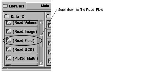
The first object you instance for your data-visualization application is Read_Field, an object that reads an AVS/Express field data file. Read_Field is located on the Main library page in the Data IO sublibrary.
Complete the steps below to create an instance of the Read_Field object.
2. Scroll through the Data IO sublibrary until you see the Read_Field icon; it will initially have parentheses around its name.
- Note: If you were to look at the underlying V code, there is an underscore between Read and Field (Read_Field). Those underscores are replaced with a space in the Network Editor.
- When you click on the icon, the object's definition is loaded into memory, and the parentheses are removed from around its name.
4. Point at the Read_Field icon, press and hold the left mouse button, and then drag the object's icon to the workspace.
- As you drag the Read_Field object, the border around the Data IO sublibrary is highlighted, and then when Read_Field object crosses over to the workspace area, the SingleWindowApp object is highlighted.
5. When the SingleWindowApp object is highlighted and the outline of the Read_Field object is displayed in the workspace area, release the mouse button.
Notice that the template of Read_Field remains in the Readers library. This means that you can create multiple instances of an object.
There are several different types of highlighting in AVS/Express:
- If you click on an object icon, the highlighting indicates that it is selected.
- As you drag a template object from one area to another, the highlighting indicates the parent object.
- For example, when you begin moving the Read_Field object, the Data I/O library is highlighted (indicating that it was the parent object.) When the Read_Field object is positioned in the SingleWindowApp object area, the SingleWindowApp object is highlighted to indicate that it will be the parent of that instance of the Read_Field object.
Examine the anatomy of the instanced Read_Field object in the Network Editior workspace. The instance's name is Read_Field. Whenever possible, AVS/Express uses the template's name as the default name for the instance. You can change an object's name, although in this tutorial you will use the default names. The colored regions are called ports. They are used for connecting objects so that data can be referenced. You will learn more about ports later.
Read_Field has three ports, one at the top (an input port) and two at the bottom (output ports). The icon to the left of the object name indicates the kind of object; Read_Field is a macro. A macro is an object that encapsulates a set of connected sub-objects.
You can easily reposition objects in the workspace:
- The mouse pointer should not be over any of the object's ports.
AVS/Express executes your application as you build it. This helps you prototype the application and verify the work you have done.
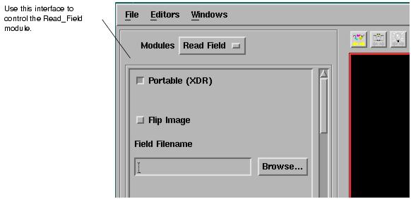
For example, when you instanced Read_Field, the object's user interface was automatically displayed through the Module Editor in the DataViewer window so you could select a data file.
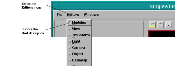
To access the Read_Field interface:
The DataViewer displays the interface for the Read_Field module:
When there is more than one module in the workspace, you can use the Modules menu to choose which interface you want to use.
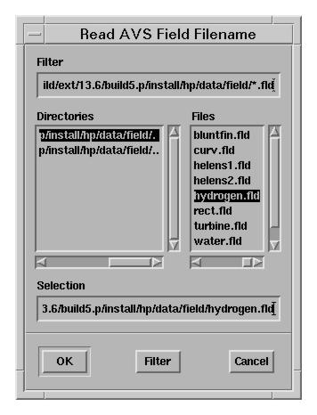
- A file-selection dialog appears. Do not select a file yet.
- The file-selection dialog disappears.
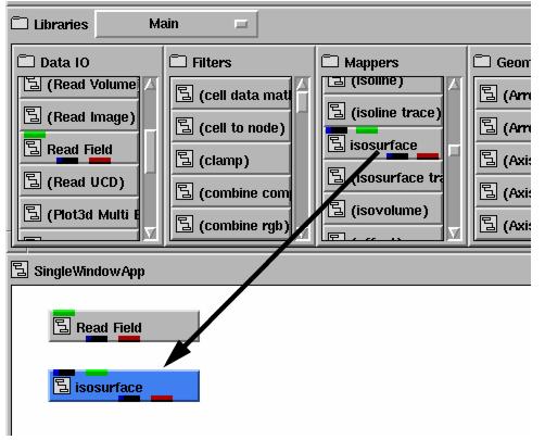
Your application requires one other object, isosurface. The isosurface object creates a surface of constant value, analogous to 3D contour lines. isosurface's user interface, accessible through the DataViewer module stack window, lets you specify the isosurface value.
1. From the Mappers library on the Main library page, instance isosurface and place it below Read_Field. You need to scroll down a bit to see it:
In AVS/Express, a connection defines a data reference. This means that the object on the input side of the connection refers to the data created by the object on the output side of the connection.
For the data-visualization application, you make two connections:
- isosurface to Read_Field so that isosurface operates on the field data produced by Read_Field
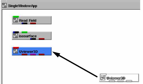
- Uviewer3D to isosurface so that the viewer displays the data produced by isosurface
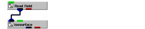
You connect objects by linking an output port of one of the objects to an input port of the other. For example, here is what Read_Field and isosurface look like when they are connected. The connection indicates that isosurface gets its data by referencing the data produced by Read_Field.
- Note: You can instance and connect the objects in any order. For example, you can instance all of the objects first, then connect them after. Or you can instance a couple of objects, connect them, instance another, and so forth. The order of execution is unaffected.
In fact the AVS/Express connections between objects are bidirectional. You will learn more about this aspect of connections in Chapter 7, Creating a New Component. See Experiment with Bidirectional Connections on page 7-27.
- Notice that several connection lines appear. These indicate possible connection paths. AVS/Express displays connections only to compatible objects.
- As you move the pointer, the Network Editor highlights (in white) the connection it will make if you release the mouse button. It also highlights (in bright green) the icons of the objects that would be connected.
- If you create a potential connection to the wrong object or port, you can cancel the connection operation by returning the mouse pointer to the output port, so that no possible connections are highlighted, before releasing the mouse button.
4. When the Network Editor highlights the connection to Read_Field's output port, release the mouse button.
- A connection line appears between Read_Field's leftmost output port and isosurface's leftmost input port.
- Note: You could have connected the objects in reverse order; that is, by dragging the mouse pointer from Read_Field's output port to isosurface's input port. It makes no difference.
If you make an incorrect connection, you can remove the connection.
You can disconnect objects in two ways:
- Point to one of the connected ports, then, holding down the left mouse button, drag the pointer to the other connected port. The Network Editor highlights in dark green the icons of the objects whose connection will be deleted. When you release the mouse button, the connection disappears.
- Point somewhere along the connection line, press and hold the right mouse button, and then select Delete Connection from the popup menu.
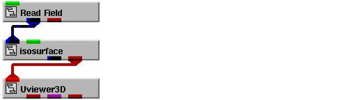
- Here is the resulting network:
Consider for a moment what ports actually mean. A port located at the top or bottom of an object exposes a subobject of the object for connection. A subobject is an object within the object. A port at the top of an object exposes a subobject for an input connection. A port at the bottom of an object exposes a subobject for an output connection.
You can see what this means by opening isosurface to see the connections to its subobjects:
1. Move the mouse pointer over isosurface, but not over a port, and hold down the right mouse button. A popup menu appears. Don't release the mouse button.
- The results are different for Visualization and Development Editon users.
- Viz/Express Edition
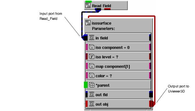
- AVS/Express displays the following subobjects and parameters:
In the Developer's Edition, you can see this view of the object by right clicking on the object and selecting Display Parameters from the popup menu.
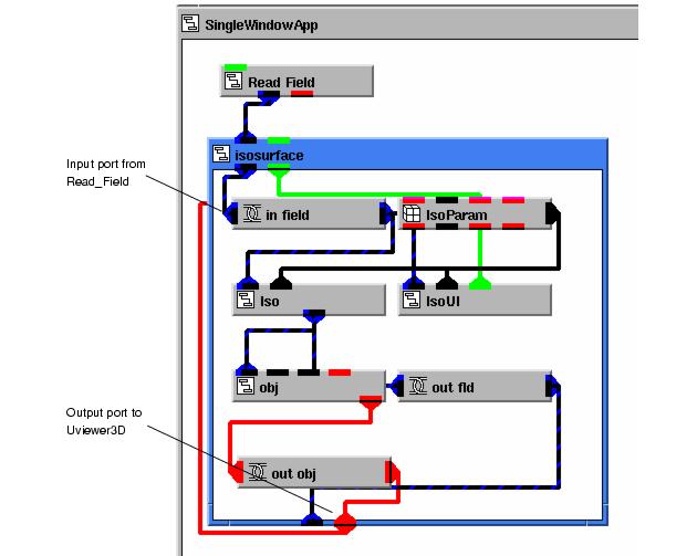
In the Developer Edition, AVS/Express expands the object to display the network of subobjects that makes up isosurface. You may need to resize the isosurface frame to see all the objects.
- In both cases, you can see that isosurface's input port-the port that you connected to Read_Field-actually leads to a subobject called in_field. Similarly, isosurface's output port-the port that you connected to Uviewer3D-actually leads to a subobject called out_obj. A port on an object's left or right side, as in the case of in_field, exposes the object itself for connection. You will work with and learn more about connections throughout this manual.
- A popup menu appears.
When closed, isosurface hides its underlying complexity. The module's ports expose only those subobjects that require a connection to external data.
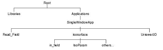
This organization of objects within objects is called the object hierarchy. In AVS/Express terminology, the objects in isosurface-in_field, IsoParam, and so forth-are called subobjects of isosurface. isosurface is their parent object. isosurface, in turn, is a subobject, or child, of SingleWindowApp.
AVS/Express maintains a single object hierarchy to which all objects belong. At the top of the object hierarchy is an object called Root. Root is not visible in the Network Editor.
Here is a small portion of the object hierarchy, with emphasis on the objects in the SingleWindowApp workspace that you have instanced:
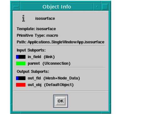
You can get information about an object's ports without opening it by using the Object Info dialog.
- The Object Info dialog appears:
- Notice that the dialog lists, among other things, the subobjects associated with the input and output ports as well as the type of data that each port expects.
In this section, you save the application.
The application that you have created to this point includes both the data-visualization network that you built, and the SingleWindowApp framework in which you built it. This is important because SingleWindowApp is responsible for displaying the DataViewer window. The SingleWindowApp workspace is also an object, a special kind called an application.
- A standard file-selection dialog appears.
You may want to create a directory located at the top level in advance so you can access it easily. For example, you might create a directory named xptutorial to hold the files you will be saving as you work through this manual.
AVS/Express saves the application as a V code text file.
In this section, you use the application you have created to view a data file.
- A file-selection dialog appears.
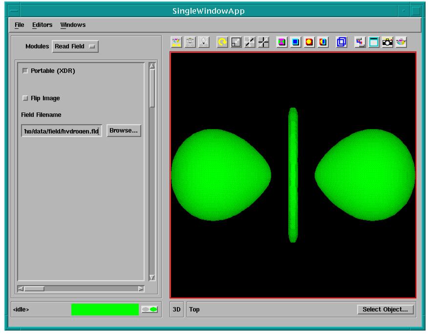
- AVS/Express executes your application's objects, highlighting each object as it executes. Read_Field reads the field data file. isosurface then creates an isosurface of that data and produces a graphics-display object, also known as the data object, since it is the visual representation of the data. Uviewer3D then renders the object and displays it in the DataViewer viewer window. AVS/Express automatically normalizes and centers the object so that it appears in the center of the view:
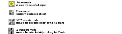
- Look at the icons at the top of the window and notice that the fourth icon from the left in the second group of icons is highlighted. The highlighting indicates the currently selected mode. This highlighted icon is the Rotate icon and it is one of the four transformation icons.
- The transformations supported in the DataViewer are scaling, translating (moving), and rotating the object in the View window. You select which type of transformation you want to perform by clicking on one of the transformation icons at the top of the viewer window. They are the fourth through seventh icons from the left:
b. Point to the image in the DataViewer window, press and hold the left mouse button, and then drag the mouse pointer downward an inch or so.
- As you do, the image is reduced. If you had moved the mouse pointer upward, the image would have been enlarged.
Uviewer3D gives you another way to transform an object: through a Transformation Editor.
b. The Transformation Editor appears in the DataViewer editor panel, replacing the Modules editor. By default the Interactor Behavior panel is displayed.
d. Try out the dials and entry fields. To move a dial, drag it with the left mouse button. To enter a value in a field, change the current value, then press Enter. You can use this interface to set the rotation of objects in the view to a precise location.
e. Press the Absolute button near the top left of the panel. Notice that the dials and fields are updated with the current location of the object. With the Transformation Editor still displayed, perform transformations once again with mouse operations. For example, rotate the object. Notice that the Transformation Editor's sliders and entry fields are updated to reflect the transformation.
- Again from the Editors menu in the DataViewer menu bar, select Modules. From the Modules option menu at the top of the panel, select isosurface. The user interface for isosurface appears.
- Notice that the current value of the iso level slider is 127.00. This means that you are producing an isosurface of data at 127.00.
- Move the iso level slider slightly. The image in the viewer window changes, reflecting the new data produced by isosurface.
In this section, you re-execute the application directly from the command line.
- AVS/Express exits after displaying a confirmation message.
- Start AVS/Express by typing the platform-specific command listed below. Depending on where you saved viz1.v, you may have to specify a pathname.
- Notice the -vcp option. This tells AVS/Express to display the V Command Processor, which it does not do automatically when you specify a V file on the command line.
- The application starts, but the Network Editor does not appear.
- For more information about starting AVS/Express, see Using AVS/Express, Chapter 2, Starting and Exiting AVS/Express
- For more information about working in the Network Editor see Using AVS/Express, Chapter 3, Working with the Network Editor.
- For detailed information on the Uviewer3D or isosurface modules see the on-line reference pages for them.