This is an archival copy of the Visualization Group's web page 1998 to 2017. For current information, please vist our group's new web page.
SNAZ Project SupportContents
IntroductionWe are working with Adam Burrows and Don Fisher at the University of Arizona in the visualization of 2D simulation results from VULCAN/2D. VULCAN/2D is a hydrodynamics code that is being used to simulate core collapse in supernovae The VULCAN simulations are part of the SciDAC Computational Astrophysics Consortium, led by Stan Woolsey, which is studying supernovae, gamma-ray bursts, and nucleosynthesis. The title of the SciDAC project is, "When Good Stars Go Bang." See Adam Burrow's Web site for more information on this research. At NERSC, this project is known as SNAZ. Initially, we developed a file format converter that converted data files in the VULCAN format to vtk files that could then be imported into the visualization program, VisIt. This work is described on SNAZ Project Support - I. This page also includes a number of 2D and 3D visualiztion examples that show:
The 3D visualizations were generated by reflecting the 2D data. Some of the images were made using AVS/Express and others were made using VisIt. The volume rendered images compare the effect of using different transfer functions (i.e., color mapping), whereas logarithmic coloring was used for some of the pseudocolor plots. The page also includes several mpeg movies showing the time evolution of the variable(s) being displayed. Development of a VisIt Database ReaderAs described on SNAZ Project Support - I, we initially developed a format converter to write the results from the VULCAN simulation into vtk format. Though this conversion was fairly straightforward, it had the disadvantage of generating one intermediate (vtk) file for each data file. Our next step was to develop a database reader (aka "plugin") for VisIt that would read the VULCAN simulation data directly into VisIt. We tested the VULCAN2D plugin on several new VULCAN datasets, and some results from one of them are shown below. In order to provide the user with some display options, the plugin reads a "plugin parameter" file that specifies the following:
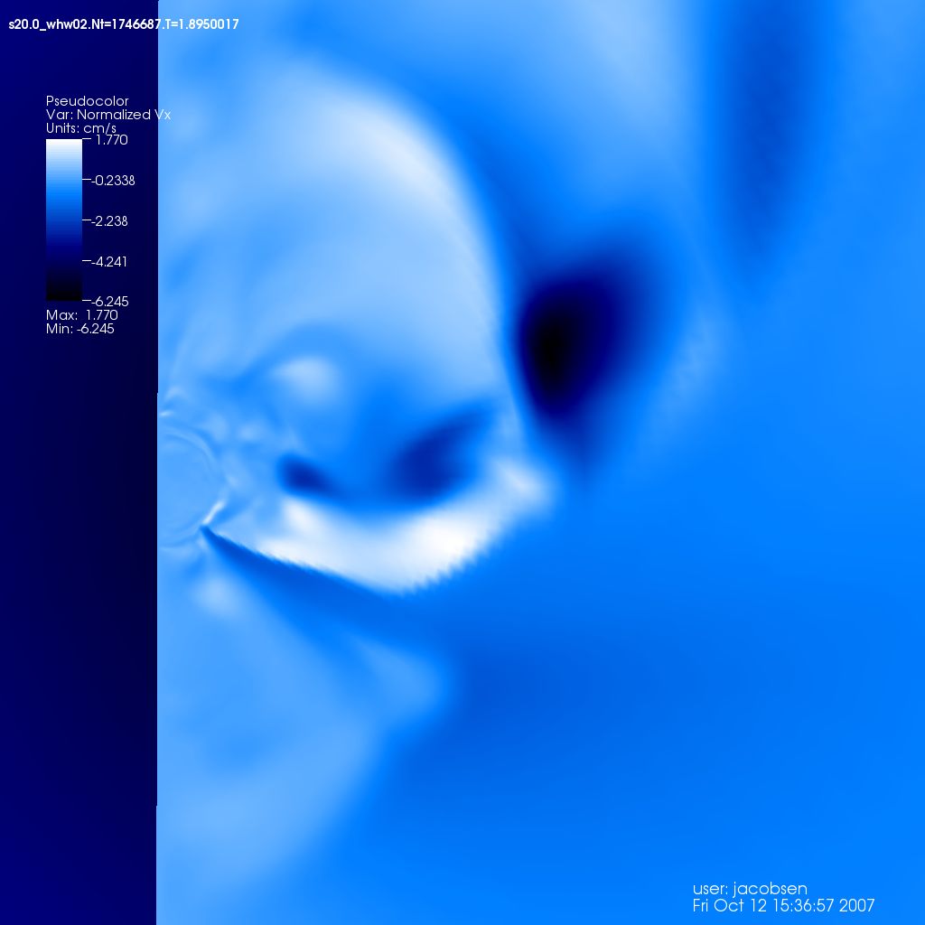
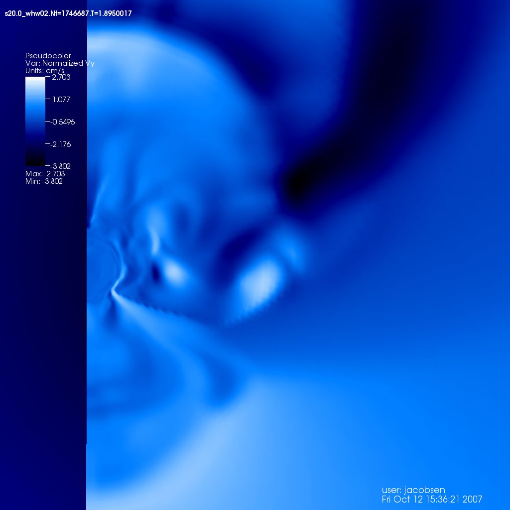
Note that VisIt has a "Reflect operator" that can be used to reflect 2D scalar data to create 3D datasets. However, as of early November 2007, the Reflect operator does not properly rotate vector fields when performing a reflection, so the VULCAN2D plugin includes the option to reflect the vector fields. Images of the 2D Velocity FieldThe velocity field for the s20.0_whw02 dataset initially is symmetric, but by the end of the simulation, displays a complicated flow pattern as shown in Images 1-3. Image 1 uses a modified reverse hot-cold color map, where finer gradations in color are used for the lower end of the range of magnitudes in order to distinguish low magnitude velocity regions from high to moderate ones. Images 2 and 3 help to distinguish the effects of the x and y components of the velocity field.
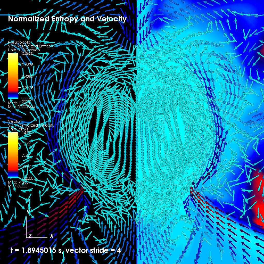
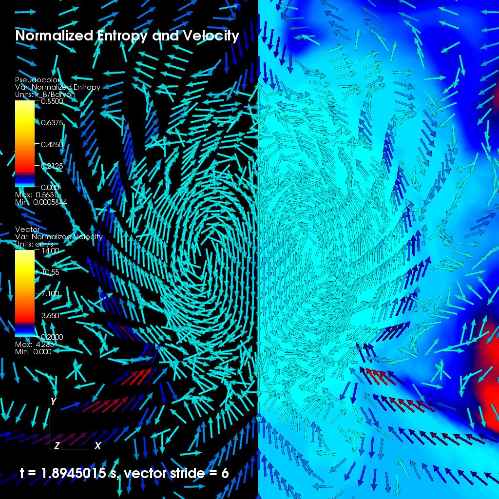
More Images of the 2D Velocity FieldImages 4-6 illustrate the dramatic effect that color map, scaling, vector stride, and thresholding have on the visualization of the vector field. The color map used for these images is quite different from the color map used for Images 1-3; for Images 4-6, a slightly different, modified hot-cold color maps have been used. In addition, the vectors have not been scaled by magnitude. Though this results in fewer areas in which vectors obscure one another, it also eliminates one important visual clue that can be used to perceive differences in magnitude. Vectors with a normalized magnitude less than 0.2 have been eliminated in Images 5 and 6, thereby revealing the structure in the inner core, which is obscured in Image 4. (Images 5 and 6 are a slightly more close-up view than Image 4.) A pseudocolor plot of the normalized entropy has been aded to the right sides of Images 5 and 6. Different strides have been used in Images 5 and 6 with the result that the motion the flow field in these two images appears to be different. More examples showing the effect of stride on the apparent motion of the flow field are on a separate page.
Notes on Making MoviesFor the mpeg movies on this page, I used the "Save movie" option in VisIt to generate a command that can be run at the command line to generate images from a VisIt "database" of files. I then use FFMPEG, which is included in the distribution of Ensight8, to assemble the images into an mpeg movie. The next step is to develop a movie 'script' using VisIt's Python interface in order add zooming, rotations, and 'fly throughs' to the animations. Next StepsOur next steps are to
| ||||||||||||||||||||