5
Macros
This chapter provides an introduction and comprehensive reference material for the Data Visualization Kit high level macros.
Note: Some of the macros described in this chapter are available only in the Developer Edition. Where this is the case, a line identifying this fact appears directly below the module name at the top of the page.
Visualization macros are macro objects that combine visualization base modules with UI objects in a structure that is convenient for building visualization networks and applications. Visualization macros have input/output ports and UI widgets that automatically appear on the Module Stack panel. You connect them using the Network Editor.
In Libraries.Main, the visualization macros are classified as follows:
Modules and macros that input data files from disk or create data. Geometries, for example, create objects such as slice planes, 2D and 3D axes, crosshairs, arrows, and diamonds, that are used by other modules to slice data, represent vector quantities, act as data probes, show data, and so forth.
Modules and macros that read data from disk are documented in this chapter.
Geometries are documented in Chapter 4, Geometries".
Modules and macros that primarily modify the field's Node_Data.
Modules that primarily modify the field's mesh.
Modules and macros that use the ip_Image data type for image processing. These are documented in Chapter 5, IP image processing macros".
Modules and macros that render data on the screen. These objects are part of the Graphics Display Kit, not the Data Visualization Kit. They are documented in the Graphics Display Kit manual.
Modules and macros that write data to disk files.
Visualization objects appear multiple times in a variety of places in the Libraries palette other than Main. To find them, use the Network Editor's Object Finder (see the User's Guide for details).
Most modules and macros report their status and their execution can be interrupted from the Module Stack Controls panel.
Most visualization modules and macros have sample networks that you can run showing how the object is properly connected within a network, and the kinds of effects it can produce on sample data.
Each reference page lists the sample networks that illustrate its use.
The examples are found in Libraries.Examples.Visualization in the Network Editor.
The reference pages for the modules include a path to the module. This path describes where you can locate the module in the network editor. Some modules belong to more than one library (for example, slice). To locate all paths to a particular module, use the Object Finder.
When determining which port on the icon corresponds to which documented item, remember that ports are documented from left to right. The first input port documented on the reference page is the leftmost port on the icon, the second input port documented is the second port from the left on the icon, and so on.
You can use a module or macro icon's Info panel to see the name and class of a port:
- With the cursor on the icon, press the right mouse button to activate the pulldown menu.
- Select Info. The first input port listed is the leftmost port on the icon, the second port listed is the second port from the left on the icon, and so on.
Visualization macros are defined in v/modules.v.
The Graphics Display Kit contains a GDmodes subobject called normals whose value specifies whether and how vertex normals are generated for Data Visualization Kit modules. The following table lists the allowed values for the normals subobject and their meanings:
GD_NORMALS_VERTEX is the default for most modules, and vertex normals are therefore generated.
However, for the following modules, the default setting is GD_NORMALS_NONE:
For more information on the GDmodes subobject, see Section 6.15, DefaultModes [page 6-51] in the Graphics Display Kit manual.
release massless particles into velocity field
advector releases a sample of zero mass particles into a field with a component that represents a velocity vector, for example, a fluid flow simulation. The particles have no initial direction or speed. The particles move through the velocity field according to the magnitude and direction of the vectors at the nodes in the volume. A forward differencing method is used to estimate the next position of each particle as a function of its current position and velocity (see the section labelled Algorithm on page 5-10).
Advection starts when you turn the Run toggle on. Advection for individual particles stops when one of the following conditions occurs:
- A particle exceeds the Max Segments value.
- The particle's velocity drops below the Min Velocity.
- The particle goes outside the field's bounds.
Advection of all particles stops when one of the following two conditions occurs:
The input is any mesh with Node_Data. The first component is used and must be a scalar or a two- or three-element velocity vector. You can use extract_component before this macro to get the component you want out of a multi-component field.
Any mesh whose coordinates represent the sample points. Meshes that are not unstructured are accepted, but a local unstructured version is generated during execution.
To create this sampling mesh you could use the plane object in Geometries.FPlane or the slice macro.
A Grid describing a glyph to represent the particles. This is simply a mesh describing the geometry of the glyph. Any mesh can be used (for example, that of a teapot), but for convenience you can use the Geometries objects to generate arrows or solid arrows, and so on
A port to connect to a user interface object that contains the macro's widgets. By default, it is connected to the default user interface object in the application in which the macro is instanced. (This default connection is not drawn.)
UIradioBoxLabel. A radio box to pick which of the input field's components to use as the velocity vector. The selection can be a one-, two-, or three-element vector. The default is the first (0th) component. If node data labels are present, they are displayed.
UIslider. An integer slider that sets the number of integration steps used within one grid "cell" to compute the streamline/particle path. The default is 2. The range is from 0 to 16.
UIslider. An integer slider that sets the total number of integration steps. When an individual particle exceeds this value, integration for it stops. The range is from 1 to 10000. The default is 256.
UIslider. An integer slider that sets the order of integration. Higher orders are more accurate, but execute more slowly. The default is 2. The range is from 1 to 4.
UIslider. A float slider. When a particle falls below this velocity, the integration process for that particle stops. The default is 0.00001. The range is from 0.0 to unbounded. You can use this to prevent wasted computation for particles barely moving, or even stationary (Min Velocity = 0).
UIradioBoxLabel. A radio box that controls whether particles are advected forward or backward from the starting sample points. The default is forward.
UIradioBoxLabel. A radio box that establishes how glyphs are rendered to represent the data values. (Glyphs are always colored by the magnitude of the data values in the component.) The choices are scalar, vector, or components:
Scale the glyph by the magnitude of the vector at that position. Also rotate the glyph in X, Y, (and Z) by the first, second, (and third) vector subcomponent values at that position. For example, a Cross3D in_probe would be rotated to reflect the vector values.
Scale the glyph in X, Y, (and Z) by the first, second, (and third) vector subcomponent values at that position. For example, a Cross3D in_probe's three lines would be individually scaled to match the vector values.
UItoggle. If off, the sizes of the glyphs are proportional to the data component values at each node. If on, all glyphs are the same size. The default is off.
UIslider. A float slider to adjust the sizes of the glyphs. The default is 1.00. The range is 0.0 to 100.00.
UIslider. A float. The time value along the original streamline continuum at which to start advection. (See DVadvect man page.) The default is 0.0.
UIslider. A float. The time value along the original streamline at which to halt advection of all particles. The default is 1.0.
UIslider. A float. The value by which to increment the time along the original streamline continuum for each advection step. The default is 0.2.
UIfieldTypein. An output only widget that displays the current time in the count from Start Time to End Time.
UItoggle. Starts or stops advection.
UItoggle. Reset Time to the value of Start Time.
UItoggle. When End Time is reached, start the advection again at Start Time.
The output is a new unstructured Mesh composed of the original mesh plus the meshes representing the particles. Its new Node_Data element's values represent the selected velocity component.
This output field is a new unstructured mesh of cell type Polyline that represents the streamlines. Its new Node_Data contains the selected element's velocity component. The output also contains a reference to the input field's xform.
This is a renderable version of the out_fld output field.
This is a renderable version of the out_fld1 output field.
advector uses precomputed streamlines (from DVstream) as particle paths. It integrates velocity along the streamlines to calculate the new position of the particles at each time step.
The streamlines are originally calculated using the Runge-Kutta method of specified order with adaptive time steps.
Libraries.Examples.Visualization.Advect
examples/advect.vrelease massless particles into Multi_Block velocity field
advect_multi_block releases a sample of zero mass particles into a field with a component that represents a velocity vector, for example, a fluid flow simulation. The particles move through the velocity field according to the magnitude and direction of the vectors at the nodes in the volume. A forward differencing method estimates the next position of each particle as a function of its current position and velocity (see "Algorithm" on page 5-15).
Advection starts when you turn the Run toggle on. Advection for an individual particle stops when one of the following conditions occurs:
- The particle exceeds the Max Segments value.
- The particle's velocity drops below the Min Velocity.
- The particle goes outside the field's bounds.
Advection of all particles stops when one of the following conditions occurs:
The input is a Multi_Block object. A Multi_Block object can be created with fields_to_mblock or Plot3D_Multi_Block. A Multi_Block object consists of an array of fields describing the data and some ancillary metadata. The first component of the fields' data is used and must be a scalar or a two- or three-element velocity vector. You can use mblock_to_fields, extract_component_ARR and fields_to_mblock before this macro to get the component you want from a multi-component Multi_Block.
Any mesh whose coordinates represent the sample points. Meshes that are not unstructured are accepted, but a local unstructured version is generated during execution.
To create this sampling mesh you could use the slice macro or the plane object in Geometries.FPlane.
A Grid describing a glyph to represent the particles. This is simply a mesh describing the geometry of the glyph. Any mesh can be used (for example, that of a teapot) but for convenience you can use the Geometries objects to generate arrows or solid arrows, and so on
A port to connect to a user interface object that contains the macro's widgets. By default, it is connected to the default user interface object in the application in which the macro is instanced. (This default connection is not drawn.)
UIslider. An integer slider that sets the number of integration steps used within one grid "cell" to compute the streamline/particle path. The default is 2. The range is from 0 to 16.
UIslider. An integer slider that sets the total number of integration steps. When an individual particle exceeds this value, integration for it stops. The range is from 1 to 10000. The default is 256.
UIslider. An integer slider that sets the order of integration. Higher orders are more accurate, but execute more slowly. The default is 2. The range is from 1 to 4.
UIslider. A float slider. When a particle falls below this velocity, the integration process for that particle stops. The default is 0.00001. The range is from 0.0 to unbounded. You can use this to prevent wasted computation for particles barely moving, or even stationary (Min Velocity = 0).
UIradioBoxLabel. A radio box that controls whether particles are advected forward (1) or backward (0) from the starting sample points. The default is forward.
UIradioBoxLabel. A radio box that establishes how glyphs are rendered to represent the data values. (Glyphs are always colored by the magnitude of the data values in the component.) The choices are:
Scale the glyph by the magnitude of the vector at that position. Also rotate the glyph in X, Y, (and Z) by the first, second, (and third) vector subcomponent values at that position. For example, a Cross3D in_probe would be rotated to reflect the vector values.
Scale the glyph in X, Y, (and Z) by the first, second, (and third) vector subcomponent values at that position. For example, a Cross3D in_probe's three lines would be individually scaled to match the vector values.
UItoggle. If off (0), the sizes of the glyphs are made proportional to the data component values at each node. If on (1), all glyphs are the same size. The default is off.
UIslider. A float slider to adjust the sizes of the glyphs. The default is 1.00. The range is 0.00 to 100.00.
UIslider. The time value along the original streamline continuum at which to start advection. (See DVadvect reference page.) The default is 0.0.
UIslider. The time value along the original streamline continuum at which to halt advection of all particles. The default is 1.0.
UIslider. The value by which to increment the time along the original streamline continuum for each advection step. The default is 0.2
UIfieldTypein. An output only widget that displays the current time in the count from Start Time to End Time.
UItoggle. Starts (1) or stops (0) advection.
UItoggle. Reset Time to the value of Start Time.
UItoggle. When End Time is reached, start the advection again at Start Time.
The output is a new unstructured Mesh composed of the original mesh plus the meshes representing the particles. Its new Node_Data element's values represent the selected velocity component.
This output field is a new unstructured mesh of cell type Polyline that represents the streamlines. Its new Node_Data contains the selected element's velocity component. The output also contains a reference to the input field's xform.
This is a renderable version of the out_fld output field.
This is a renderable version of the out_fld1 output field.
advect_multi_block uses precomputed streamlines (from DVstream) as particle paths. It integrates velocity along the streamlines to calculate the new position of the particles at each time step.
The streamlines are originally calculated using the Runge-Kutta method of specified order with adaptive time steps.
generate a bounding box of a 3D structured field
bounds generates lines and/or surfaces that indicate the bounding box of a 3D structured field. This is useful when you need to see the shape of an object and the structure of its mesh. For example, isosurface can produce a fairly cryptic shape floating without context in space, but when combined with bounds, you see the isosurface within its surrounding mesh.
The input field must contain any type of structured mesh (mesh type Mesh_Struct, Mesh_Unif or Mesh_Rect). Node_Data can be present, but is only used if you switch on Data.
A port to connect to a user interface object that contains the macro's widgets. By default, it is connected to the default user interface object in the application in which the macro is instanced. (This default connection is not drawn.)
UIradioBoxLabel. Selects which of the input field's components to send to the output, if Data is also turned on. The default is the first (0th) component. If node data labels are present, they are displayed.
UItoggle. When on, draws a wireframe around the perimeter extents of the mesh. The default is on.
UItoggle. When on, causes the Imin/Imax, Jmin/Jmax, Kmin/Kmax controls to produce a wireframe representation of the mesh grid at that plane. The default is off.
UItoggle. When on, causes the Imin/Imax, Jmin/Jmax, Kmin/Kmax controls to produce a solid face representing the location of that plane extent. The default is off.
UItoggle. When on, each of these switches displays the grid (Edges turned on) or plane (Faces turned on) on one of the six faces of the hull. Imin/Imax draw a mesh or face showing the 2D slice of field objects with the minimum/maximum index value in the first dimension. Jmin/Jmax draw a mesh or face showing the 2D slice of field objects with the minimum/maximum index in the second dimension. Kmin/Kmax control the third dimension. The default for all is off.
UItoggle. When on, makes bounds copy the selected component's Node_Data values at node points along the output mesh to the output field. Because the data is present, the bounds lines can be colored by the interpolated data values of the selected Node_Data component. Otherwise, the lines display as white in the renderer. The default is off.
The output field contains a new unstructured Mesh object with cell type Polyline (Edges selected) and/or Quad (Faces set) representing the bounds. If Data was selected, the output field also contains a Node_Data that is the selected component's values at nodes on the output mesh.
This is a renderable version of the output field.
Libraries.Examples.Vizualization.Crop
examples/crop.vproduce a Point mesh representing geometric centers of each cells
cell_centers module produces a mesh containing Point cell set, each point of which represents a geometrical center of a corresponding cell in the input mesh. The coordinates of cell centers are calculated by averaging coordinates of all the nodes of a cell. The number of nodes in the output mesh is equal to number of cells in the input mesh. If the input mesh contains Cell_Data it becomes a Node_Data in the output mesh with each node values equal to corresponding cell value. You can use this module to create a position mesh for the glyph module (see Section 5.45, glyph [page 5-105]).
The input must contain any type of mesh.
The output field contains a new mesh that consists of points representing geometrical centers of a corresponding cells in the input mesh.geoetric centers. It also may contain a Node_Data that corresponds to Cell_Data in the input mesh.
This is a renderable version of the output field.
Libraries.Examples.Visualization.Cylinder_Plot_Unif
examples/cyl_plot_unif.vperform arbitrary math operations on cell-based data
cell_data_math performs arbitrary math operations on up to four cell-based datasets. You can use any operation or expression that can be specified in the V language to operate on the data. The expression you enter may use #1, #2, #3, and #4 to stand for the four input fields.
Mesh+Cell_Data. Input to math expression. Use "#1" in the expression to refer to this field.
Mesh+Cell_Data. Input to math expression. Use "#2" in the expression to refer to this field.
Mesh+Cell_Data. Input to math expression. Use "#3" in the expression to refer to this field.
Mesh+Cell_Data. Input to math expression. Use "#4" in the expression to refer to this field.
A port to connect to a user interface object that contains the macro's widgets. By default, it is connected to the default user interface object in the application in which the macro is instanced. (This default connection is not drawn.)
UItext. Math expression to perform on the cell data of the inputs. All V language expressions are valid; use #1 through #4 to refer to the input fields. For example, the expression sqrt(#1 * 10 + sin(#2/#3))computes a function of the first three inputs.
Mesh+Cell_Data. Contains the result of applying the given expression to the input field(s).
Renderable object. Renderable version of out_fld.
convert Cell_Data to Node_Data
cell_to_node converts Cell_Data to Node_Data. It is necessary to convert cell-based data to node data when the visualization modules or macros selected do not process cell-based data.
Note: All nodes referenced by a cell with a NULL value will have their Node_Data set to NULL.
The input is a field with an unstructured Mesh and Cell_Data.
A port to connect to a user interface object that contains the macro's widgets. By default, it is connected to the default user interface object in the application in which the macro is instanced. (This default connection is not drawn.)
UIoptionBoxLabel. A series of buttons that let you select which components in the input field to convert to Node_Data. You can select multiple components. If the Cell_Data contains multiple cell_sets, the conversion is performed on the specified components in each cell_set.
UIslider. An integer that sets the order of interpolation. Allowed values are:
A node's value is computed by interpolating values using distances from the node to the adjoining cell centroids.
The output is a reference to a merged object that contains the new Node_Data, plus the existing Mesh and Cell_Data.
This is a renderable version of the output field.
Libraries.Examples.Visualization.Cell_Data
examples/celld.vcreate plot of blocks based on the height (value) of a 2D field
city_plot creates a block on each node of the input mesh. The color and height (out of the grid) of the block are determined independently by selectable input data components at that node. The lower left (min X and Y) corner of the block is at the node's coordinate, so the city plot extends over the dimensions of the field by one block width (in X) and length (in Y), because the block at (maxX, maxY) extends from that point to (max_x + scale_x * x spacing, max _y + scale_y * y spacing).
Mesh_Unif + Node_Data + Dim2. The 2D field to be plotted.
A port to connect to a user interface object that contains the macro's widgets. By default, it is connected to the default user interface object in the application in which the macro is instanced. (This default connection is not drawn.)
UIradioBoxLabel. Selects which component of the input to map to the height of the block at that point of the grid.
UIradioBoxLabel. Selects which component of the input to map to the color of the block at that point of the grid.
UItoggle. When turned on (1), the heights of the blocks are normalized to a constant value set by the height scale, and the glyph_comp is ignored.
UIslider. Scales the input height value by this amount. If normalize is on, this value becomes the height of the blocks. Height is measured in the coordinate system of the input field.
UIslider. Scales the X size of each block relative to the size of that block's cell width. scale_x of 1 means the block takes up the full width of the cell and abuts the next block (in X); scale_x of 0.5 means the block takes up 1/2 the width of the cell.
UIslider. Scales the Y size of each block relative to the size of that block's cell width. scale_y of 1 means the block takes up the full length of the cell and abuts the next block (in Y); scale_y of 0.5 means the block takes up 1/2 the length of the cell.
The output field is an unstructured Mesh of cell type Quad containing the blocks.
Renderable object corresponding to out_fld.
Libraries.Examples.Visualization.City_Plot
examples/city_plot.vclamp minimum and maximum values of data
clamp transforms the values of the selected field component subcomponent as follows:
- If Above max_value is set, any value above max value is set to max value.
- If Below min_value is set, any value below min value is set to min value.
- Otherwise, the values are not changed.
If Above max_value and Below min_value are on, the output field's selected component values are all in the range of min value <= value <= max value. Null data values are not affected.
Note the difference between clamp and the threshold macro:
- threshold sets values outside the range to a specified null value.
- clamp sets values outside the range to min value and/or max value.
The input field must contain a Node_Data object. If a Mesh is present, it is passed along untouched as a reference in the output field. The field's data components can be scalar or vector.
A port to connect to a user interface object that contains the macro's widgets. By default, it is connected to the default user interface object in the application in which the macro is instanced. (This default connection is not drawn.)
UIradioBoxLabel. Selects which of the input field's components to clamp. The default is the first (0th) component. If node data labels are present, they are displayed.
UIslider. If the selected data component is non-scalar, you can pick which subcomponent to clamp. The range is 0 (first subcomponent) to the number of subcomponents. The default is 0.
UItoggle. When on, clamps data above the max value. The default is off.
UItoggle. When on, clamps data below the min value. The default is on.
UItoggle. When on, clamp recalculates the data's minimum and maximum values. The default is off.
UIslider. Double precision floating point sliders that set the min and max values. The default is set to the input field component's node data minimum and maximum. The range shown is from the component's node data minimum to its maximum. The double precision value is converted to the data type of the input field before use. Two decimal points of precision are given.
The output field contains a new Node_Data object that is the clamped component. If a Mesh was present, the output field contains a reference to that mesh.
If a Mesh was present, this is a renderable version of the output field. Otherwise, rendering objects generate an error.
Libraries.Examples.Vizualization.Clamp
examples/clamp.vtake components from two different fields to make a new n-component field
combine_comp takes the selected components from the first input field, and the selected components from the second input field, creating a new output field with n components. The output field's mesh, if present, comes from the first input field. For example, selecting the second components from each of the fields (a, b, c) and (d, [e, f, g]) results in the field (b, [e, f, g]).
This input field must contain any mesh with Node_Data object. If a mesh is present, it is passed along untouched as a reference in the output field. The field's data components can be scalar or vector.
This input field must contain a Node_Data.
A port to connect to a user interface object that contains the macro's widgets. By default, it is connected to the default user interface object in the application in which the macro is instanced. (This default connection is not drawn.)
UIoptionBoxLabel. Select which of the input fields' components to combine. The default for both is the first (0th) component. If node data labels are present, they are displayed.
The output field is a Node_Data that is an array of references to the two selected Node_Data components. If a mesh was present, the output field contains a reference to that mesh.
This is a renderable version of the output field.
combines a mesh and cell data array to produce a field
combine_mesh_cell_data combines a mesh and and a cell data array. The in_data object represents the values of some dataset at the cells of a field, while the in_mesh represents the locations and connectivity of that mesh's nodes and cells. The in_mesh object should have one cell set to which cell data is added. The in_data can be a primitive array of any type: byte, int, float, etc. If in_data is a one dimensional array, the scalar cell data is created. The dimension of this array should be the same as ncells in in_mesh. If it is two-dimensional array, the low dimension is used for data veclen and the high dimension should be the same as ncells in in_mesh.
This macro simplifies the process of generating field; it is used to combine the output of a mesh mapper with the raw array of cell data.
prim. This array can be of any primitive type (int, float. etc.)
Mesh+Cell_Data. Mesh with cell data.
Output renderable object corresponding to out.
combine a mesh and some node data to produce a field
combine_mesh_data combines a mesh and some node data. A Node_Data object represents the values of some dataset at the node points of a field, while the Mesh represents the locations of that field's nodes in space.
This macro simplifies the process of generating field data by reducing the amount of data you must supply to create a field. Usually this macro is used to combine the output of a mesh mapper with the output of one or more data mappers.
Mesh. This input is the Mesh part of the result.
Node_Data. This input is the Node_Data part of the result.
Mesh+Node_Data. This contains the two inputs, merged.
Output renderable object corresponding to out.
Section 5.72, radius_data, rgb_data, argb_data, node_colors, node_normals, node_uv, node_uvw, pick_data [page 5-171]
combine different Node_Datas into one Node_Data with multiple components
combine_node_datas combines several sets of node data (for example, radius and color data), into one node dataset that can be incorporated into a field. It makes each node_data into a component of the output Node_Data. If an input has more than one component, all its components are inserted into the output in order, at the same level as the other components from other inputs.
A Node_Data object represents the values of some dataset at the node points of a field, while the Mesh represents the locations of that field's nodes in space.
These macros simplify the process of generating field data by reducing the amount of data you must supply to create a field. Usually the output of one of these macros is combined, using combine_mesh_data, with the output of one of the mesh mapper macros to create a field.
Node_Data[]. This input is an array of Node_Data objects. Each one becomes one or more components of the output Node_Data.
Node_Data. This contains all the components from the inputs.
Section 5.72, radius_data, rgb_data, argb_data, node_colors, node_normals, node_uv, node_uvw, pick_data [page 5-171]
combine three scalars into an RGB image
combine_rgb combines three scalar 2D, 2-space byte input fields into an RGB image. This macro is similar to combine_vect except it only works on exactly three 2D 2-space uniform byte fields, and it sets the resulting node data ID to tell the renderer that it is an RGB image.
Mesh_Unif+Dim2+Byte+Space2+Node_Data. This field represents the red channel of the image.
Mesh_Unif+Dim2+Byte+Space2+Node_Data. This field represents the green channel of the image.
Mesh_Unif+Dim2+Byte+Space2+Node_Data. This field represents the blue channel of the image.
Renderable object corresponding to out_fld.
combine n scalar components into a single n-vector component
combine_vect takes all the selected data components, which must be scalar, and produces a single output data component that is the specified veclen long. For example, selecting the first and third components of (a, b, c, [e,f,g]) results in the field ([a, c]).
The input field must contain a Node_Data object. If a mesh is present, it is passed along untouched as a reference in the output field. The field's data components must include at least two scalar components.
A port to connect to a user interface object that contains the macro's widgets. By default, it is connected to the default user interface object in the application in which the macro is instanced. (This default connection is not drawn.)
UIslider. Sets the number of scalar components to combine and the out_fld's single component veclen. The default is 3. The range is 1 to 4.
UIoptionBoxLabel. Selects which of the input field's components to combine. If you select vector components, only the first vector subcomponent is extracted. If node data labels are present, they are displayed. The default is the first three components.
The output field contains a new Node_Data that is a data array of references to the selected components in the original input Node_Data. It has one component with veclen equal to the specified veclen. If a mesh was present, the output field contains a reference to that mesh.
If a mesh was present, this is a renderable version of the output field. Otherwise, rendering objects generate an error.
Libraries.Examples.Visualization.Advect
examples/advect.v
Libraries.Examples.Visualization.Curl
examples/curl.v
Libraries.Examples.Visualization.Glyph_Interp
examples/glh_intp.vconcatenate elements of several arrays or individual scalar primitives into an array
These modules concatenate elements of several arrays or individual scalar primitives into an output array. Input arrays may have any dimensionality, but are treated as 1-dimensional, in memory order.
Input arrays can have different total sizes; the size of the output array is the sum of the sizes of the input arrays. The output array contains all elements from the first array, followed by all elements from the second array, and so on.
For example, this can be used to create an XYZ coordinate array from separate X, Y, and Z arrays.
prim[]. One of the input arrays or scalar primitives.
prim[]. One of the input arrays or scalar primitives.
prim[]. One of the input arrays or scalar primitives.
prim[]. One of the input arrays or scalar primitives.
prim[]. The output array containing the concatenated data.
create an isovolume bounded by two isosurfaces (3D) or isolines (2D)
contour creates a field that is the volume bounded by two isosurfaces (if the field is 3D) or two isolines (if the field is 2D).
For example, you could set the min level and max level isosurfaces to densities found just outside a bone. When combined, the isovolume produced would be the bone itself.
The isosurfaces or isolines are colored by the first map component selected. All of the selected map components are in the Node_Data of the output field.
Note: The contour module does not generate vertex normals by default. For more details, see Section 5.1.8, Vertex normal generation [page 5-4].
The input is any mesh with Node_Data. A 2D mesh will produce isolines. A 3D mesh produces isosurfaces. At least one of the components must be scalar.
A port to connect to a user interface object that contains the macro's widgets. By default, it is connected to the default user interface object in the application in which the macro is instanced. (This default connection is not drawn.)
UIradioBoxLabel to pick which component to isosurface/isoline. The selected component must be scalar or the message "iso: first component is not scalar" is written to stderr. The default is the first (0th) component. If node data labels are present, they are displayed.
UIoptionBoxLabel to pick components that will be written to the output field. In addition, the first selected component will be mapped onto the isosurface/isoline (for example, map pressure value onto a density isosurface). The selection does not have to be scalar. The default is the first (0th) component. If node data labels are present, they are displayed. Where the isosurface/isoline does not exactly intersect a node, the data value is linearly interpolated based on the surface's distance from the adjacent nodes.
UIslider. Float sliders that set the minimum and maximum isosurface/isoline values, between which data is extracted. The default is 0.0. The range is from the minimum data value in the selected contour component to the maximum data value in the selected contour component. The data type of the slider is converted to the data type of the node data before use.
The output field is an unstructured Mesh of cell type Tri (3D) or Line (2D) that represents the contour volume. Its Node_Data is the values within the volume. The surface values are interpolated along the isosurface/lines.
This is a renderable version of the output field.
contour uses the Marching Cubes algorithm to construct the isosurfaces/isolines. See W. Lorensen and H. Cline, "Marching Cubes: A High Resolution Surface Reconstruction Algorithm." Computer Graphics 21(4) (SIGGRAPH Proceedings, 1987), July, 1987, pp. 163-169.
This algorithm has a known limitation. There are cases where there are two possible paths that the isosurface could take through a cell, and only one is the correct path. If isosurface picks the wrong path, a discontinuity appears as a hole in the surface.
Libraries.Examples.Vizualization.Contour
examples/cont.v
Libraries.Examples.Vizualization.Contour_2D_Unif
examples/cont2uni.v
Libraries.Examples.Vizualization.Cylinder
examples/cyl.vcopy a mesh to a selected region of an output array of meshes
copy_ROI copies an input mesh, typically created by one of the Graphics Display Kit's interactive drawing modules (for example, ClickSketch, ContinuousSketch) to an array of output meshes. This module is a quick way to create an array of ROIs that correspond to a volume. The ROIs can subsequently be edited individually by using the EditMesh module.
The size of the output mesh array is determined by using a reference input field. The input mesh may be copied to a region of the output mesh array by using the start and stop parameters appropriately.
The reference input field must be uniform, 3D and have node data. This field is used to dimension the output array of meshes
The input mesh to be copied into the output mesh array.
UIfieldTypein. Start index into the output mesh array.
UIfieldTypein. Start index into the output mesh array.
UItoggle. When set, Run starts the copy operation. It is automatically cleared when the copy operation is completed.
The output array of meshes. This array is dimensioned by the reference input field. Depending on the values of Start and Stop, all or part of the output
Libraries.Examples.Visualization.Tile_ROI
Libraries.Examples.Visualization.Display_Vol_ROIextract a subset of a structured field
crop reduces the size of a structured field by extracting the data within a specified range of its dimensions. The process is analogous to "cropping" a photographic image. Typical uses are to eliminate uninteresting portions of the data and to increase processing speed by reducing the amount of data.
The input must contain a structured mesh object (Mesh_Struct, Mesh_Rect, or Mesh_Unif), and a Node_Data object. The mesh can be 1D, 2D, or 3D.
A port to connect to a user interface object that contains the macro's widgets. By default, it is connected to the default user interface object in the application in which the macro is instanced. (This default connection is not drawn.)
UIsliders. Used to set crop dimensions. I min, J min, and K min set the lower bound array index in their respective dimensions; I max, J max, and K max set the upper bound array index in their respective dimensions. All default to 0 (min) and the maximum dimension of the mesh (max), so that the default is no cropping. Their range is from 0 to the maximum dimension of the Mesh for I, J, and K. All three pairs of controls appear no matter what the dimensionality of the input Mesh. Use just the controls meaningful for the input data.
The output field contains a new Mesh_Struct and a new Node_Data associated with the cropped region.
If the input was a Mesh_Rect or a Mesh_Unif, its points array (extents) are modified to retain the mesh's position in space.
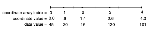
For example, the following 1D field has a points array (extents) from 0 to 49.
You crop the field using an I min of 30 and an I max of 49. The output field has coordinate indices from 0 to 19 and a points array from 30 to 49.
The output field also contains a new Node_Data that has the data within the cropped region.
This is a renderable version of the output field.
Libraries.Examples.Vizualization.Crop
examples/crop.vcompute the curl of a vector field
curl computes the curl of a vector field with any mesh type.
The input must be a field with any type of mesh and Node_Data. At least one of the Node_Data's components must be a three-element vector.
A port to connect to a user interface object that contains the macro's widgets. By default, it is connected to the default user interface object in the application in which the macro is instanced. (This default connection is not drawn.)
UIradioBoxLabel. A radio box to pick which component of in_field to use to compute the curl. You must pick a three-element vector component. The default is the first (0th) component. If node data labels are present, they are displayed.
The output field contains a new Node_Data that has a three-element float at each node representing the curl. Its mesh is a reference to the input mesh.
This is a renderable version of the output field.
The algorithm used to compute the curl in structured meshes is a finite difference approximation based on a central difference scheme. For unstructured meshes, the function is based on the cell shape functions and their derivatives.
In both cases, where the input is the vector function:

The equation used to compute the curl is:

Libraries.Examples.Vizualization.Curl
examples/curl.vcut off a portion of a field on one side of cutting plane
cut lets you cut (divide) a field into two pieces, and output one of the pieces. You position an arbitrarily-oriented cutting plane within the field, and select which side of the cutting plane you wish to output. Output is generated every time the cutting plane moves.
Note: The cut module does not generate vertex normals by default. For more details, see Section 5.1.8, Vertex normal generation [page 5-4].
The input must be a field with any type of 2D or 3D mesh and any type. It may optionaly have node and/or cell data components
The cutting plane. This is generated by the plane object found in Geometries.FPlane. The plane object has its own Plane Transformation panel that controls plane rotation, translation, and scale, as well as controls to specify its size when it is connected to the default user interface object in the application in which the macro is instanced.
A port to connect to a user interface object that contains the macro's widgets. By default, it is connected to the default user interface object in the application in which the macro is instanced. (This default connection is not drawn.)
UIoptionBox. A selection to pick which components of in_field's node data (if prsent) to send to the output field. You can pick more than one or none. The default is the first (0th) component. If node data labels are present, they are displayed.
UIoptionBox. A selection to pick which components of in_field's cell data (if present) to send to the output field. You can pick more than one or none. The default is the first (0th) component. If cell data labels are present, they are displayed.
UItoggle. Picks which side of the slice plane to send to the output field. The default is on.
UIslider. A float slider that moves the plane through the field perpendicular to the plane. Though the Plane Transformation panel has X, Y, and Z transformation controls, it is usually easier to use plane's controls to orient and size the plane, but use this plane distance control to move the plane. cut generates output whenever the slice plane moves. The default distance is 0.0 and the range is the extents of the field.
The output field contains a new mesh object that is the subset of the original mesh. It has the same type as the input mesh. It may have node and/or cell data containing the selected components. Its extents are set to retain the position of the cut section of the field in space.
This is a renderable version of the output field.
Libraries.Examples.Vizualization.Cut
examples/cut.vmacro that includes cut and cutting plane
cut_plane is a macro that includes the cut macro and an FPlane cutting plane object. It cuts away the part of a field above or below the arbitrarily-oriented cutting plane, revealing the internal structure.
Note: The cut_plane module does not generate vertex normals by default. For more details, see Section 5.1.8, Vertex normal generation [page 5-4].
The input field to cut. You can specify any 2D or 3D mesh with any primitive type of node data and/or cell data.
A port to connect to a user interface object that contains the macro's widgets. By default, it is connected to the default user interface object in the application in which the macro is instanced. (This default connection is not drawn.)
int[]: UIoptionBoxLabel. Select which node data component(s) are to be mapped onto the resulting mesh
int[]: UIoptionBoxLabel. Select which cell data component(s) are to mapped onto the resulting mesh.
UItoggle. Selects whether the part of the mesh above (1) or below (0) the cutting plane is removed. Above is in the positive Z direction of the cutting plane.
UIslider. The plane at which the field is cut can be offset from the plane described by the internal plane object, which is what is transformed by the Plane Transform Editor. The offset is in the direction of the Z axis of the cutting plane. Note that if you offset the cutting plane from the plane object, the plane object output still shows the position of the plane object, not the actual cutting plane.
UIbutton. This button brings up the plane transform editor panel, which you can use to transform the cutting plane to any arbitrary orientation.
Mesh[+Node_Data] [+Cell_Data]. The mesh with the part above or below the cutting plane removed. It may have node and/or cell data from the part of the input field.
Plane_Mesh. A mesh containing the cutting plane. This is simply a rectangle spanning the minimum and maximum of the first two dimensions of the field. It is transformed to lie at the correct spatial location.
Renderable object corresponding to out_fld.
Renderable object corresponding to out_plane.
show 3D uniform field as a texture-mapped sliced solid
cut_texture3D shows a 3D uniform field as a solid, with one slice cut off to reveal the interior structure. The slice plane can be moved through the volume perpendicular to the X, Y, and Z axes. Output is generated every time the slice plane moves.
cut_texture3D differs from interp_texture3D in the following ways:
- Its slicing plane can only be moved orthogonal to the X axis.
- It can display the exterior surfaces of the volume.
Texture mapping is much faster than the sampling techniques used by DVslice, particularly for large datasets. The point sampling done by the texture mapping technique is always done at the resolution of the data; thus, differences in data values within a small area are not obscured, as they can be with DVslice.
The input must be a field with a Mesh_Unif, Space3, Dim3, and Node_Data.
The slicing plane. This is generated by the Plane object found in Geometries.Plane or Geometries.FPlane. The plane object has its own Plane Transformation panel that controls plane rotation, translation, and scale, as well as controls to specify its size when it is connected to the default user interface object in the application in which the macro is instanced.
A colormap to provide the texture map. From Libraries.Main.Fields.Data.colormap.
A port to connect to a user interface object that contains the macro's widgets. By default, it is connected to the default user interface object in the application in which the macro is instanced. (This default connection is not drawn.)
UIoptionBoxLabel. An option box to pick which components of in_field to texture map. You can pick more than one. The components must be scalar. The default is the first (0th) component. If node data labels are present, they are displayed.
UItoggle. Picks which side of the slice plane to send to the output field.
UIslider. A float slider that moves the plane through the field perpendicular to the plane. Though the Plane Transformation panel has X, Y, and Z transformation controls, it is usually easier to use plane's controls to orient and size the plane, but use this plane distance control to move the plane. cut_texture_3D generates output whenever the slice plane moves. The default distance is 0.0 and the range is the extents of the field.
The output field contains a new mesh object that is the subset of the original mesh. It has the same type as the input mesh. It has a new Node_Data containing the texture mapping u, v, w values. Its points array (extents) is set to retain the position of the volume of the field in space.
This is a renderable version of the output field.
cut_texture3D creates its picture of the volume data using 3D texture mapping. In this method, the boundary of the volume has three values, u, v, w, associated with each of its vertices. Where the slice planes intersect this volume, u, v, w values are computed for the vertices of the resulting solid. These values are attached to the vertices of the output object. Viewers use the u, v, w information to create the texture-mapped rendering.
Libraries.Examples.Vizualization.Cut_Texture
examples/cut_txt.vproduce a set of cylindrical glyphs that allow you to visualize two dimensional table data
cylinder_plot_unif allows you to visualize two dimensional node data that can be thought of as a table having some number of columns and rows. Each column in the table is represented with a cylinder glyph. A cylinder is divided in either vertical or angular direction into a number of segments equal to the number of rows in the column. Each segment is scaled (in either vertical or angular direction) proportionally to the data value of the row. The height or radius of each cylinder can optionally be scaled by the total value of the column (sum of all rows). The sides of the cylinder can optionally be colored by the total column value.The resultant image looks like a 3D pie chart.
The input must contain a 2-dimensional uniform mesh (Mesh_Unif+Dim2) plus Node_Data.
This port is optional. It is a grid describing the location of the cylinders. If nothing is connected to this port, the module will use coordinates of in_field to position the cylinders. This port is useful, for example, to position a cylindrical glyph at certain locations on a map.
A port to connect to a user interface object that contains the macro's widgets. By default, it is connected to the default user interface object in the application in which the macro is instanced. This default connection is not drawn.
UIradioBoxLabel. Radio buttons to pick which input Node_Data component to use to create cylinders. The default is the first (0th) component.
UItoggle. Indicates whether to use angular of vertical segmentation for each cylinder. The default is off (angular segmentation).
UItoggle. Indicates whether a height for each cylinder (representing a column of an input table data) is scaled by the total value of the column (sum of all rows).
UItoggle. Indicates whether a radius for each cylinder (representing a column of an input table data) is scaled by the total value of the column (sum of all rows).
UItoggle. Indicates whether the sides of each cylinder (representing a column of an input table data) are colored by the total value of the column (sum of all rows).
UIfield. Represents a default radius value for all cylinders. If "scale radius by total" is set to on, this value is used as the scale for radii of the cylinders.
UIfield. Represents a scale value for heights for the cylinders. If "scale height by total" is set to off, this value is used as the height for all the cylinders.
UIslider. An integer value that represents the total number of sub-divisions for each cylinder. This number is used to control the graphical accuracy of the cylinders shape - the higher the value, the more accurate the cylinder is drawn (with a corresponding increase in drawing time). If this value is set to 4 you will get rectangular (4-sided) blocks instead of a cylinder. The default is 36.
UIslider. Controls the start angle for the first segment in a case when vertical segmentation is off (angular segmentation is specified). Changing this angle is equivalent to rotating all cylinders around their vertical axis. The default is 0.
UIsliders. Float sliders to adjust the color of the cylinder side. These colors are used only when "color sides by total" is off. The defaults are 1.0.
The output field contains cylindrical glyphs.
This is a renderable version of the output field.
Libraries.Examples.Visualization.Cylinder_Plot_Unif
examples/cyl_plot_unif.vperform mathematical operations on fields using V expressions
data_math performs mathematical operations on one to four input fields. You type in any valid V expression, and use the OutDataType selection box to pick the data type for the result.
The input field(s) must be a field with any type of mesh and Node_Data. You can use from 1 to 4 inputs. When typing the expression, you refer to them as #1, #2, #3, and #4.
data_math uses the first (0th) component of each field. Operations between two fields require that their components be the same length (nnodes must be equal) and both components have the same veclen.
A port to connect to a user interface object that contains the macro's widgets. By default, it is connected to the default user interface object in the application in which the macro is instanced. (This default connection is not drawn.)
UItext. Any valid V mathematical expression. Do not enclose in quotes or terminate with a semi-colon (that is, ";"). The following expression calculates the vector magnitude of the 0th component of input fields 1, 2, and 3 (treating the combination of those three fields as a vector):
sqrt(pow(#1,2) + pow(#2,2) + pow(#3,2))
UIradioBoxLabel. Radio buttons to set the data type in which the computation will be performed. Each input's 0th component Node_Data is first converted to that type, the computation is performed in that type, and the output Node_Data is in that type. The choices are char, byte, short, int, float, and double. The default is float.
The output field contains a new Node_Data that has the result of the computation. Its mesh is a reference to the input mesh of in_field1.
This is a renderable version of the output field.
For more information on expressions, see the section on value expressions in the Developer's Reference manual.
display a slice from a volume and display a mesh from an array of meshes
display_vol_ROI displays a single slice from a volume and the associated ROI from an array of meshes. The proper slice and ROI are selected by using the slice input parameter.
The input field must be uniform, 3D, and have node data. A slice is taken from this field and displayed as an image.
The input array of meshes. A slice is taken from the array and displayed.
UIslider. The index into both the input field and array of meshes used to extract the data for display.
Graphics Display Kit DefaultObject. This is a renderable object that can be connected directly to one of the Graphics Display Kit's viewers.
Libraries.Examples.Visualization.Display_Vol_ROI
compute the divergence of a vector field
divergence computes the divergence of a vector field with any mesh type.
The input must be a field with any type of mesh and Node_Data. At least one of the Node_Data's components must be a three-element vector.
A port to connect to a user interface object that contains the macro's widgets. By default, it is connected to the default user interface object in the application in which the macro is instanced. (This default connection is not drawn.)
UIradioBoxLabel. A set of radio buttons to pick which component of in_field to use to compute the divergence. You must pick a three-element vector component. The default is the first (0th) component. If node data labels are present, they are displayed.
The output field contains a new Node_Data that has a scalar float value at each node representing the divergence. Its mesh is a reference to the input mesh.
This is a renderable version of the output field.
The algorithm that computes the divergence in structured meshes is a finite difference approximation based on a central difference scheme. For unstructured meshes, the function is based on the cell shape functions and their derivatives.
In both cases, where the vector node data component is:

The equation used to compute the divergence is:

Libraries.Examples.Vizualization.Div
examples/div.vresample a field to reduce (or increase) its size
downsize resamples a field using a scaling factor. When the factor is greater than 1, downsize reduces the size of the field, saving processing time and memory by "thinning out" the data. When the factor is less than 1, downsize increases the size of the field by duplicating data.
The following steps describe how downsize works. For each dimension i (X, Y, and Z),
2. Round dims_out to the nearest whole integer.
Note that the two endpoints are always preserved in the output data and the extents of the input field are preserved in the output field.
3. Calculate the ratio of the intervals between nodes dims_in: dims_out and calculate new array indices.
5. Use the node data and coordinates in the input field that are found by these index values as the node data and coordinates for the output field.
Note that throughout the process, the actual node data values and coordinate values are irrelevant. All that is manipulated are the indices into these arrays.
For example, given a factor of 1.2 and the following 1D input field:
 3. The number of intervals in dims_in is 4 and the number of intervals in dims_out is 3, so the ratio of the intervals between nodes dims_in: dims_out is 4 /3 or 1.333. Therefore, the four indices for dims_out are 0, 1.333, 2.666, and 3.999.
5. The result of using the coordinates and node data in the input field at these index values as the coordinates and node data for the output field is: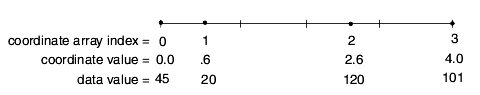
The input must contain a structured mesh object (Mesh_Struct, Mesh_Rect, or Mesh_Unif), and a single Node_Data object. The mesh can be 1D, 2D, or 3D.
A port to connect to a user interface object that contains the macro's widgets. By default, it is connected to the default user interface object in the application in which the macro is instanced. (This default connection is not drawn.)
UItoggle. When on, the downsize factor sliders are constrained to integers rather than floats. The default is on.
Float UIsliders to specify the scaling coefficient. The output field's values (and coordinates for irregular data) are:
dims_out[i] = dims_in[i] / factor [i]
where i cycles through the dims of the field, either 1D, 2D, or 3D.
Note: factors < 1 make the output field larger. For example, a factor of .5 doubles the size of the output field.
You control the factor for each dimension separately. The default for all factors is 8. The range for all factors is 0.0 to 12.0.
All three controls appear no matter what the dimensionality of the input data. You only use the controls that are meaningful for the input data.
The output field contains a new structured mesh of the same type as the input mesh, and a new Node_Data object containing the data associated with the downsized region.
The output mesh's points array (extents) will occupy the same "space" as the input field's Mesh.
This is a renderable version of the output field.
Libraries.Examples.Vizualization.Downsize
examples/down.v
Libraries.Examples.Visualization.Mirror_Scale
examples/mirr_scl.vinteractively draw lines on an object in a viewer
draw_line lets the user interactively draw polylines over an object in a viewer window.
The coordinates of the picked point. This red input port should connect to a renderer's picked_obj red output port.
A port to connect to a user interface object that contains the macro's widgets. By default, it is connected to the default user interface object in the application in which the macro is instanced. (This default connection is not drawn.)
UItoggle. When on, the user is using the left mouse button to select a series of points on the object. Lines are drawn between each point. The default is on.
UItoggle. When on, the user wants to select a new "first" point and begin drawing a new series of lines. When off, the user is in the middle of drawing a series of lines and any left mouse button click is a line endpoint. The default is off.
The output is an unstructured mesh of cell type Polyline. Each cell is one line segment in the drawing.
This is a renderable version of the output field.
perform 3D texture mapping on a 3D uniform field
excavate_brick3d is a technique for visualizing 3D uniform volume data. The volume is displayed with an X, Y, and Z slice plane. The slice removes a rectangular subvolume of the field, revealing the structures inside.
Texture mapping is much faster than the sampling techniques used by slice, particularly for large datasets. Texture mapping's point sampling is done at the resolution of the data; thus, differences in data values within a small area are not obscured as they can be with slice.
Note: The excavate_brick3D module does not generate vertex normals by default. For more details, see Section 5.1.8, Vertex normal generation [page 5-4].
The input is a reference to a Mesh_Unif, Dim3 field with scalar byte Node_Data.
A colormap to provide the texture map. From Libraries.Main.Fields.Data.colormap.
A port to connect to a user interface object that contains the macro's widgets. By default, it is connected to the default user interface object in the application in which the macro is instanced. (This default connection is not drawn.)
UIsliders that set the X, Y, Z position of their respective slice planes. The default is the mid-point of the input field's dimensions. The range is the field's dimensions.
UItoggles. These select whether the excavating cube should be positioned on the positive or negative axis for each of the X, Y, and Z dimensions. When on, the cube is positioned on the negative axis. The default is off.
UItoggle. When off, only the excavating cube is drawn. When on, a texture map of the bounding faces of the volume is also drawn. The default is off.
The output is a new Mesh and Node_Data. u, v, w textures are added.
This is a renderable version of the output field.
excavate_brick3D creates its picture of the volume data using 3D texture mapping. In this method, the boundary of the volume has three values, u, v, w, associated with each of its vertices. Where the slice planes intersect this volume, u, v, w values are computed for the vertices of the resulting solid. These values are attached to the vertices of the output object. Viewers use the u, v, w information to create the texture-mapped rendering.
Libraries.Examples.Vizualization.Excavate_Brick: examples/excvt.v
explode individual transformations of each field in the input array of fields
explode_fields takes each input field in the input array and translates it away from the common center of all the fields, which is computed by finding the midpoint of the bounding box. You can set the amount of translation via parameters. The grid and data for the input fields are not modified, only their transformation matrices.
Mesh[]. An array of fields to transform.
A port to connect to a user interface object that contains the macro's widgets. By default, it is connected to the default user interface object in the application in which the macro is instanced. (This default connection is not drawn.)
UIslider. A value specifying how much to scale the translation away from the center in the X direction. This value is in units of the bounding box of the original array of fields.
UIslider. A value specifying how much to scale the translation away from the center in the Y direction. This value is in units of the bounding box of the original array of fields.
UIslider. A value specifying how much to scale the translation away from the center in the Z direction. This value is in units of the bounding box of the original array of fields.
Mesh[]. The transformed input fields.
Renderable object corresponding to out_fld.
Libraries.Examples.Visualization.Explode_Fields
examples/explode.vcreate an array of fields from a single field based on material properties of cell sets
Each cell set in a field has an associated properties array. You may use this array to store anything related to the cell set, but it is commonly used to store material properties of the cells in the cell set.
explode_materials splits up the field into an array of fields based on the values of a particular element of the properties array. The same array index is used to look up the value in the properties array of each cell set. Each cell set with a distinct value of that property goes into a separate output field. Whether the values are equal is all that is significant, the actual values are not significant.
Note that this macro compares floating point numbers for equality; you are responsible for ensuring that the values in the material property array are bit-for-bit equal or not equal, as desired.
Mesh. This mesh is split apart into multiple meshes on the output, according to the selected property value of each cell set.
A port to connect to a user interface object that contains the macro's widgets. By default, it is connected to the default user interface object in the application in which the macro is instanced. (This default connection is not drawn.)
UIslider. Selects which element of each cell set's material properties array to use to split the input. All cell sets' arrays use the same index.
Mesh[]. An array of meshes, with other data merged from the input field.
GroupObject. Group of renderable objects corresponding to out_fld.
Libraries.Examples.Visualization.Explode_Field
examples/explode.vextract external edges of a field to reveal inside objects
external_edges produces a wireframe representation of the outside of an unstructured mesh. You use it when you want to see objects produced by other modules that are inside an unstructured mesh (isosurfaces, streamlines, probes, and so on) while still being able to see the enclosing skeletal shape of the mesh.
The input need only contain a mesh of any sort. Unstructured meshes pay attention to the max edge angle UIslider using DVext_edge to produce their picture. Structured meshes (Mesh_Struct, Mesh_Rect, and so on) cause DVbounds to be used, generating a simple hull of the mesh.
A port to connect to a user interface object that contains the macro's widgets. By default, it is connected to the default user interface object in the application in which the macro is instanced. (This default connection is not drawn.)
UIslider. A float slider that controls the accuracy of the boundary representation on the base of the angle between two adjoining faces in unstructured meshes. All edges that have an angle less than this value are represented in the output field. The range is 0.0 to 180.0. The angle used is calculated as edge_angle*3.14/180.0. The default is 5.0.
This parameter is ignored in structured meshes.
The output is a field containing a new unstructured Mesh of cell type Line representing the input mesh's exterior. If Node_Data was present in the input field, this output field also contains a reference to that Node_Data.
This is a renderable version of the output field.
Libraries.Examples.Visualization.Advect
examples/advect.v
Libraries.Examples.Visualization.Cut
examples/cut.v
Libraries.Examples.Visualization.Isosurface
examples/isos.v
Libraries.Examples.Visualization.Probe
examples/probe.v
Libraries.Examples.Visualization.Stream
examples/stream.v
Libraries.Examples.Visualization.Glyph_Interp
examples/glh_intp.v
extract external faces of a field for faster rendering
external_faces produces a mesh that represents just the exterior, visible faces of an unstructured mesh. It saves memory and greatly speeds rendering because all of the unstructured mesh's many interior, hidden nodes and cells are not represented.
Note: The external_faces module does not generate vertex normals by default. For more details, see Section 5.1.8, Vertex normal generation [page 5-4].
The input need only contain a mesh of any sort. Unstructured meshes pay attention to the max edge angle UIslider using DVext_edge to produce their picture. Structured meshes (Mesh_Struct, Mesh_Rect, and so on) cause DVbounds to be used, generating a simple hull of the mesh.
A port to connect to a user interface object that contains the macro's widgets. By default, it is connected to the default user interface object in the application in which the macro is instanced. (This default connection is not drawn.)
The output is a field containing a new unstructured Mesh of cell types Quad and Tri representing the input mesh's exterior. If Node_Data was present in the input field, this output field also contains a reference to that Node_Data.
This is a renderable version of the output field.
Libraries.Examples.Visualization.Cut
examples/cut.v
Libraries.Examples.Visualization.Isoline
examples/isol.v
Libraries.Examples.Visualization.Isovolume
examples/isov.v
Libraries.Examples.Visualization.Offset
examples/offset.vextract one cell_data component from each Cell_Data cell_set
extract_cell_component extracts one cell_data component from each Cell_Data cell_set. If there are multiple Cell_Data cell_sets, the same component is extracted from each cell_set. extrract_cell_component is the cell data equivalent of extract_component for node data.
Since the renderer draws just the first component it finds in each cell_set, you use extract_cell_component to obtain the right component from a multi-component Cell_Data field.
The input is a field with a Mesh and Cell_Data.
A port to connect to a user interface object that contains the macro's widgets. By default, it is connected to the default user interface object in the application in which the macro is instanced. (This default connection is not drawn.)
UIradioBoxLabel. A series of radio buttons to pick which single component to extract. If there are multiple Cell_Data cell_sets, the same component is extracted from each cell_set. If labels are present, they are displayed.
The output is a reference to a merged object that contains the new Cell_Data, plus references to all other unchanged objects in the input Mesh.
This is a renderable version of the output field.
Libraries.Examples.Visualization.Cell_Data
examples/celld.vextract a single data component from a field
extract_component extracts a single data component from any Node_Data. For example, selecting the fourth component of the field (a, b, c, [e, f, g]) results in the single-component vector field ([e, f, g]).
The input field must contain any mesh and Node_Data objects.
A port to connect to a user interface object that contains the macro's widgets. By default, it is connected to the default user interface object in the application in which the macro is instanced. (This default connection is not drawn.)
UIradioBoxLabel. Radio buttons to pick which data component to send to the output field. The default is the first (0th) selection. If node data labels are present, they are displayed.
The output contains a reference to the original mesh, with new Node_Data consisting of a reference to the single extracted component in the input Node_Data. Effectively, you have "extracted" a reference to one component of the input Node_Data.
This is a renderable version of the output field.
Libraries.Examples.Applications.IsoApp
extract selected coordinate components from mesh, after transforming
extract_coordinate_array extracts a 1D array containing the X, Y and/or Z components of the mesh's coordinates after being transformed by the mesh's transformation matrix. If X and Y are selected, it outputs X0, Y0, X1, Y1, and so on. Note that the output coordinates are not the same as the coordinates of the mesh itself; they are transformed, so they are in "world coordinates", as you would see them in the viewer.
A port to connect to a user interface object that contains the macro's widgets. By default, it is connected to the default user interface object in the application in which the macro is instanced. (This default connection is not drawn.)
UIoptionBoxLabel (X, Y, Z). Selects which coordinate components to extract.
prim[]. An array containing the extracted components.
extract selected component as an array from selected node data component
extract_data_array extracts a 1D array containing the selected component of the node data.
Node_Data. The input Node_Data object from which to extract the component array.
A port to connect to a user interface object that contains the macro's widgets. By default, it is connected to the default user interface object in the application in which the macro is instanced. (This default connection is not drawn.)
UIoptionBoxLabel. Selects which data component to extract.
prim[]. An array containing the extracted component.
string. The label of the selected component.
create a mesh without any data
extract_mesh outputs the same mesh as the input, but with no node data (nnode_data=0).
Mesh+Node_Data. The output mesh is copied from this input.
Mesh. Contains only the mesh part of the input field.
Renderable object corresponding to out_fld.
extract a scalar data element from a field's vector component
extract_scalar extracts a single scalar data element from a vector component of a field with Node_Data. For example, selecting the second vector element of the fourth component of the field (a, b, c, [e, f, g]) returns the field (f).
The input field need only contain Node_Data. One of its components should be a vector. If a mesh is present, it is passed through unchanged as a reference in the output field.
A port to connect to a user interface object that contains the macro's widgets. By default, it is connected to the default user interface object in the application in which the macro is instanced. (This default connection is not drawn.)
UIradioBoxLabel. Radio buttons to pick which of the components to display in the vector component selection below. The default is the first (0th) selection. If node data labels are present, they are displayed.
A selection to pick which vector element of a component to extract.
The output is a field with a new Node_Data consisting of the extracted vector element. If a mesh was present in the input field, it is included in the output field as a reference to the original mesh.
If a mesh was present, this is a renderable version of the output field. Otherwise, rendering objects generate an error.
produce a mesh with cells extruded in the Z direction based on their cell data values and optionally shrunk relative to their geometric centers
extrude_cells creates a new mesh, each cell of which is extruded in Z direction based on the selected height data (cell data) component. Optionally, cells can be shrunk relative to their geometric center (which is a point computed by averaging coordinates for all nodes in a cell). The height of extrusion is controlled by the height scale parameter. Shrink option and shrink scale is controlled by the shrink cells and shrink factor parameters. The sides of an extruded cell can optionally be created and colored based on the draw skirts and color skirts parameters.
The input must contain any type of mesh plus Cell_Data.
A port to connect to a user interface object that contains the macro's widgets. By default, it is connected to the default user interface object in the application in which the macro is instanced. (This default connection is not drawn.)
UIradioBoxLabel. Radio buttons to pick which input Cell_Data component to use as a height value for each cell. The default is the first (0th) component. If cell data labels are present, they are displayed.
UIslider. A float slider to adjust the height of extruded cells. The default is 1.0.
UItoggle. If on, the module computes new coordinates for the extruded cell's nodes based on the shrink factor value that specifies the scale relative to the geometric centers of each cell. The default is off.
UIslider. A float slider that adjusts the factor by which cells are scaled. The value of scale factor specifies scale relative to the geometric centers of each cell and can vary from 0 to 1, a value of 0 producing totally shrunken cells, and a value of 1 producing full size cells. The default is 0.8. The range is 0.0 to 1.0.
UItoggle. If on, the sides (skirts) of extruded cells are created. The default is on.
UItoggle. If on, the sides (skirts) of extruded cells are colored. The default is
off.The output field contains a new mesh that is created by extruding and optionally shrinking cells in the input field. It also contains a Cell_Data that was present in the input field.
This is a renderable version of the output field.
Libraries.Examples.Visualization.Extrude_Cells
examples/extrude.vconvert an array of fields to a Multi_Block object
fields_to_mblock takes an array of fields and converts it to a Multi_Block object by adding the ancillary information kept by the Multi_Block object.
Mesh_Struct+Node_Data+Cell_Data_Struct. The input array of fields.
Multi_Block. The resulting multiblock dataset.
Libraries.Examples.Visualization.Multi_Block
examples/mblock.vfilter 1D data by convolving with a specified filter kernel array
filter_1D takes as its input an object that has a Node_Data subobject and performs filtering (convolution) of data values based on an array of kernels. The kernels array can be a float array of any size. The module internally normalizes the kernels array so that the sum of its elements always equals one.
filter_1d outputs the input mesh with new node data containing the convolved values.
The first output value comes from overlaying the middle element of the kernel with the first data value and performing the sum of products, and so on.
Mesh+Node_Data. The 1D field containing the data to filter.
float[]. Array of floats describing the filter kernel. This array is convolved with the in_field data to produce the output. Note that this array is automatically normalized so the sum of its values is 1.
A port to connect to a user interface object that contains the macro's widgets. By default, it is connected to the default user interface object in the application in which the macro is instanced. (This default connection is not drawn.)
UIradioBoxLabel. Selects which component of the data to filter.
Mesh+Node_Data. Contains the filtered data.
Renderable object corresponding to out_fld.
take an array of glyphs as input and output glyphs at nodes using node data as an index into the glyph array
geo_glyph takes an input field and an array of glyphs, and draws one glyph at each node location of the in_field. The glyph drawn is selected by using the data at that node as an index into the glyph array.
If normalize is off, floating point values are converted to integers by truncation. If normalize is on, the data range is mapped to the number of glyphs so that each glyph represents the same fraction of the data range.
If the data is out of the bounds of the glyph array, the minimum or maximum glyph is drawn, as appropriate.
The glyphs' colors are determined by the color parameters unless the glyphs themselves provide node data for coloring, and their size is scaled by the scale parameter. Their orientation is unchanged.
Mesh+Node_Data. The field on which the glyphs are plotted.
Mesh[]. The array glyphs to plot.
A port to connect to a user interface object that contains the macro's widgets. By default, it is connected to the default user interface object in the application in which the macro is instanced. (This default connection is not drawn.)
UIslider. Scales glyph size (X, Y and Z).
UIslider. Sets color for glyphs.
UIslider. Sets color for glyphs.
UIslider. Sets color for glyphs.
UItoggle. When on (1), the range of the data is matched to the number of glyphs so that each glyph represents an equal part of the range. When off (0), the data is used directly as an index into the glyph array.
Mesh+Node_Data. Contains the output glyphs.
Renderable object corresponding to out_fld.
Libraries.Examples.Visualization.geo_glyph
examples/g_glyph.vproduce a geometric object (glyphs) at nodal locations of an input field
glyph places a geometrical object at each node of an input field so that node locations are easily identified. The glyph can be sized and colored according to the selected data component at each node. If the glyph is an arrow in a vector field, for example, it generates a hedgehog.
The input must contain any type of mesh plus Node_Data.
Grid. This is simply a mesh describing the geometry of the glyph. Any mesh can be used (for example, that of a teapot) but for convenience you can use the Geometries such as Arrow1 (wireframe arrow), Arrow2 (solid arrow), or Cross3D (XYZ crosshairs) to generate the glyph.
A port to connect to a user interface object that contains the macro's widgets. By default, it is connected to the default user interface object in the application in which the macro is instanced. (This default connection is not drawn.)
UIradioBoxLabel. Radio buttons to pick which input Node_Data component to use to scale and distort the glyph, as controlled by Mode. The default is the
first (0th) component. If node data labels are present, they are displayed.
UIradioBoxLabel. Radio buttons to pick which input Node_Data component to use to color the glyph. If map component is equal to glyph component and the map component is a vector, the color represents the magnitude of the vector. If node data labels are present, they are displayed. The default is the first (0th) component.
UIradioBoxLabel. A radio box that establishes how glyphs are rendered to represent the data values. The choices are:
Scale the glyph set by glyph component by the magnitude of the vector at that position. Also rotate the glyph in X, Y, (and Z) by the first, second, (and third) vector subcomponent values at that position. For example, a Cross3D in_probe would be rotated to reflect the vector values.
Scale the glyph set by glyph component in X, Y, (and Z) by the first, second, (and third) vector subcomponent values at that position. For example, a Cross3D in_probe's three lines would be individually scaled to match the vector values.
UItoggle. If off, the sizes of the glyphs are proportional to the magnitude of the data component values at each node. If on, all glyphs are the same size. The default is off.
UIslider. A float slider to adjust the sizes of the glyphs. The default is 1.0. The range is -10 to 10.
The output field contains a new unstructured mesh (mesh type Mesh) that is the meshes of all the glyphs. It also contains a new Node_Data consisting of the magnitude of the selected component's data values if map component is a vector, or the value of the map component if the map component is a scalar.
This is a renderable version of the output field.
Libraries.Examples.Visualization.Glyph_Interp
examples/glh_intp.v
Libraries.Examples.Visualization.Advect
examples/advect.v
Libraries.Examples.Visualization.Probe
examples/probe.vcompute the vector gradient of a vector field
gradient computes the vector gradient of a field with any mesh type.
The input must be a field with any type of mesh and Node_Data. At least one of the Node_Data's components must be a scalar.
A port to connect to a user interface object that contains the macro's widgets. By default, it is connected to the default user interface object in the application in which the macro is instanced. (This default connection is not drawn.)
UIradioBoxLabel. Radio buttons to pick which component of in_field to use to compute the gradient. You must pick a scalar component. The default is the first (0th) component. If node data labels are present, they are displayed.
The output field contains a new Node_Data that has a three-element vector float value at each node representing the gradient. Its mesh is a reference to the input mesh.
This is a renderable version of the output field.
The algorithm used to compute the gradient in structured meshes is a finite difference approximation based on a central difference scheme. For unstructured meshes, the function is based on the cell shape functions and their derivatives.
In both cases, the equation used to compute the gradient is:

Libraries.Examples.Vizualization.Grad
examples/grad.vinterleave elements of several arrays into a 2D array
These modules interleave elements from several arrays into a 2D output array. The input arrays may have any dimensionality, but they are treated as 1D, in memory order. All input arrays should have the same total size. The output array contains one element from each array in order, followed by the next element from each array, and so on.
For example, this can be used to create an XYZ coordinate array from separate X, Y, and Z arrays.
prim[]. One of the input arrays.
prim[]. One of the input arrays.
prim[]. One of the input arrays.
prim[]. One of the input arrays.
prim[][N]. The output array containing the interleaved data.
samples cell data of one field at the node locations of another "probe" field
interp_cell_data uses the node coordinates specified in the input mesh (in_probe) as a set of sample points for the in_field. For each sample point, it locates the cell containing that point in the in_field, and uses the (possibly vector) value of the given component in that cell as the node data in the output field.
If there is no cell in in_field containing a given sample point, a null data value is used.
Mesh+Cell_Data. This field is sampled at the locations determined by the nodes of in_probe.
Mesh. The node coordinates of this field define the sample points for interpolating in_field.
A port to connect to a user interface object that contains the macro's widgets. By default, it is connected to the default user interface object in the application in which the macro is instanced. (This default connection is not drawn.)
UIradioBoxLabel. Which data component to interpolate.
Mesh+Node_Data. The sampled field data.
Renderable object corresponding to out_fld.
use coordinates from a probe mesh as sample points to interpolate data in a field
interp_data uses the coordinates specified in an input mesh (in_probe) as a set of sample points for a field. It takes each set of coordinates in the mesh (the sample points), locates these same coordinates in the input field, then calculates what the interpolated data value of the selected component would be at that exact location based on the values of the same component in the adjacent nodes.
The input is any mesh type with Node_Data.
Any mesh whose coordinates represent the sample points.
To create this sampling mesh you could, for example, use the plane object in Geometries.Plane, Geometries.FPlane, or the slice macro.
A port to connect to a user interface object that contains the macro's widgets. By default, it is connected to the default user interface object in the application in which the macro is instanced. (This default connection is not drawn.)
UIoptionBoxLabel. A set of option buttons to pick which data components of the input field to interpolate. The default is the first (0th) component. If node data labels are present, they are displayed.
The output is a field that is a reference to the merge of the input probe's in_probe mesh, and a new Node_Data object with values consisting of the interpolated component values.
This is a renderable version of the output field.
Structured fields use trilinear interpolation. Unstructured fields use shape function interpolation.
Libraries.Examples.Vizualization.Glyph_Interp
examples/glh_intp.v
Libraries.Examples.Applications.StreamApp
examples/stream_l.vshow an arbitrarily oriented and shaped texture mapped sample of a 3D uniform field
interp_texture3D creates a texture mapped picture of the surface of any mesh where it intersects a 3D uniform field. The sampling object can be moved through the volume in any direction. Output is generated every time the sampling object moves.
interp_texture3D differs from cut_texture3D in the following ways:
- It can texture map any object, not just a slicing plane. This sampling object can be moved in any direction with its Transformation Editor panel, not just orthogonal to the X axis.
- It only displays the texture mapped sampling object, not the exterior surfaces of the volume.
Texture mapping is much faster than the sampling techniques used by the slice modules, particularly for large datasets. The point sampling done by the texture mapping technique is always done at the resolution of the data; thus differences in data values within a small area are not obscured as they can be with slice.
The input must be a field with a Mesh_Unif, Space3, Dim3, and Node_Data.
The sampling object. This is generated by one of the Geometry objects such as Plane or Box. The sampling object should come with its own Transformation panel that controls object rotation, translation, and scale, as well as controls to specify its size when it is connected to the default user interface object in the application in which the macro is instanced.
A colormap to provide the texture map. From Libraries.Main.Fields.Data.colormap.
A port to connect to a user interface object that contains the macro's widgets. By default, it is connected to the default user interface object in the application in which the macro is instanced. (This default connection is not drawn.)
The output field contains a new mesh object that is the texture mapped slice. It has the same type as the input mesh. It has a new Node_Data containing the texture mapping u, v, w values.
This is a renderable version of the output field.
interp_texture3D creates its picture of the volume data using 3D texture mapping. In this method, the boundary of the volume has three values, u, v, w, associated with each of its vertices. Where the slice planes intersect this volume, u, v, w values are computed for the vertices of the resulting solid. These values are attached to the vertices of the output object. Viewers use the u, v, w information to create the texture-mapped rendering.
Libraries.Examples.Vizualization.Interp_Texture3D
examples/intrptxt.vcreate a surface of constant value at a picked probe location
iso_probe creates a surface of a given level value in a field at a probe position. This probe position is picked either interactively with the left mouse button, or specified through a Transformation Editor. This surface is, in effect, a 3D contour.
This isosurface of one component is colored by the value of another component, for example, the isosurface of density colored by temperature. The selected iso_probe component must be scalar. You use iso_probe when you want to see a graphic depiction of the locations of a particular data value at a particular location in a 3D field.
The input is any mesh with Node_Data. The mesh can be of any defined type (Mesh, Mesh_Struct, Mesh_Unif, Mesh_Rect). At least one of the components must be scalar.
Grid. A glyph to represent the probe object. This is simply a mesh describing the geometry of the glyph. Any mesh can be used, for example, that of a teapot, but for convenience you can use the predefined glyphs in Geometries (for example, Cross3D or Arrow1) to generate the mesh.
This input connects to a renderer's picked_obj red output port. It informs iso_probe which object has been picked to probe.
A port to connect to a user interface object that contains the macro's widgets. By default, it is connected to the default user interface object in the application in which the macro is instanced. (This default connection is not drawn.)
UIradioBoxLabel to pick which component to isosurface. The selected component must be scalar or the message "iso: first component is not scalar" is written to stderr. The default is the first (0th) component. If node data labels are present, they are displayed.
UIradioBoxLabel to pick a component that will map onto the isosurface, for example, map pressure value onto a density isosurface. The selection does not have to be scalar. The default is the first (0th component). If node data labels are present, they are displayed. Where the isosurface does not exactly intersect a node, the data value is linearly interpolated based on the surface's distance from the adjacent nodes.
UItoggle. If off, the size of the probe is proportional to the data component values at each node. If on, the probe is the probe scale size. The default is off.
UIslider. A float slider to adjust the size of the probe. The default is 1.0. The range is -10.00 to 10.
UIslider. A float slider. This is an output parameter only-it displays the value of the data at the probe's location. Where the probe does not fall exactly on a node, the value is interpolated from the values of adjacent nodes.
Note that the value displayed is accurate if the selected component was a scalar. If it was a vector, you see only the value of that component's first vector element.XformEditor. A transformation editor used to place the probe within the input field if you do not want to use the left mouse button to point and click a position.
The output field is an unstructured Mesh of cell type Tri that represents the 3D contour surface. Its Node_Data is the interpolated values of the map_component component along the isosurface.
This output is of marginal utility. It contains the mesh of the probe object and Node_Data that is the value of the data at the probe's current location.
This is a renderable version of the output field.
This is a renderable version of the probe object.
iso_probe uses the Marching Cubes algorithm to construct the isosurface. See W. Lorensen and H. Cline, "Marching Cubes: A High Resolution Surface Reconstruction Algorithm." Computer Graphics 21(4) (SIGGRAPH Proceedings, 1987), July, 1987, pp. 163-169.
This algorithm has a known limitation; where there are two possible paths that the isosurface could take through a cell, only one is the correct path. If isosurface picks the wrong path, a discontinuity appears as a hole in the surface.
Libraries.Examples.Vizualization.Iso_Probe: examples/isop.v
create contour lines of constant value
isoline creates contour lines of a given level value or values in a field. The contour lines are colored by the level value. The selected component must be scalar. You use isoline when you want to see a graphic depiction of the locations of a particular data value in a field.
The input is any mesh with Node_Data. The mesh must be a surface (nspace = 2). The surface can exist in 2D or 3D. No checking is done to ensure that the mesh is 2D. 3D meshes do not generate output. At least one of the components must be scalar.
A port to connect to a user interface object that contains the macro's widgets. By default, it is connected to the default user interface object in the application in which the macro is instanced. (This default connection is not drawn.)
UIradioBoxLabel. A set of radio buttons to pick which component to compute the isolines for. The selected component must be scalar or the message "isoline: first component is not scalar" is written to stderr. The default is the first (0th) component. If node data labels are present, they are displayed in the UIradioBox.
UIslider. Number of isolines to produce. The lines are evenly spaced between the min and max levels. Default number is 10.
UIslider. Float slider to set the minimum isoline level. The default is the selected component's min * 0.7 + max * 0.3. The range is from min to max. The data type of the slider is converted to the data type of the node data before use.
UIslider. Float slider to set the maximum isoline level. The default is the selected component's min * 0.3 + max * 0.7. The range is from min to max. The data type of the slider is converted to the data type of the node data before use.
UItoggle. When on, the isolines are colored by the data value. The default is on.
The output field is a new unstructured Mesh of cell type Line that represents the contour lines. It has a new Node_Data whose value at each line is the level value of that line.
This is a renderable version of the output field.
For each "cell" of the field, a straight line is created connecting locations on the cell's edges with an interpolated value equal to the iso level. The interpolation is linear.
Libraries.Examples.Visualization.Isoline
examples/isol.vcreate a local line of constant value at a picked probe location
isoline_trace is similar to isoline. It creates a line of a given level value in a 2-space field at a probe position. This probe position is picked interactively with the left mouse button or specified through a Transformation Editor. This line is, in effect, a 2D contour.
isoline_trace differs from isoline in that it does not isoline the entire volume of the field. Rather, beginning from the picked position, it builds an isoline by checking the values of adjacent cells until either no more adjacent cells have the same value, it hits the limits of the field, or the line is closed. Thus, isoline_trace creates local isolines.
The isoline is colored by the value of the selected iso component. That component is also written to the output Node_Data.
The input is any Mesh_Struct (Mesh_Struct, Mesh_Rect, or Mesh_Unif) with Node_Data. The mesh must be a surface (nspace = 2). The surface can exist in 2D or 3D. No checking is done to ensure that the mesh is 2D. 3D meshes do not generate output. At least one of the components must be scalar.
Grid. This input is a Grid representing any kind of probe object. Such objects are found in Geometries, such as Arrow, or Cross3D. In turn, the probe macro icon's red input port must connect to the renderer's picked_obj red output port.
A port to connect to a user interface object that contains the macro's widgets. By default, it is connected to the default user interface object in the application in which the macro is instanced. (This default connection is not drawn.)
UIradioBoxLabel to pick which component to isosurface. The selected component must be scalar or the message "iso: first component is not scalar" is written to stderr. The default is the first (0th) component. If node data labels are present, they are displayed.
UIslider. This widget is output only. A float slider that reports the value for which the isoline is being drawn.
The output field is an unstructured Mesh of cell type Line that represents the 2D contour lines. Its Node_Data is the interpolated values of the iso component along the isolines.
This is a renderable version of the output field.
isoline_trace uses the Marching Cubes algorithm to construct the isosurface. See W. Lorensen and H. Cline, "Marching Cubes: A High Resolution Surface Reconstruction Algorithm." Computer Graphics 21(4) (SIGGRAPH Proceedings, 1987), July, 1987, pp. 163-169.
This algorithm has a known limitation. There are cases where there are two possible paths that the isosurface could take through a cell, and only one is the correct path. If isosurface picks the wrong path, a discontinuity appears as a hole in the surface.
create a surface of constant value
isosurface creates a surface of a given constant value level in a field. This surface is, in effect, a 3D contour. This isosurface of one node data component can be colored by the value of another node data or cell data component (for example, the isosurface of density colored by temperature). The selected iso component must be scalar. You use isosurface when you want to see a graphic depiction of the locations of a particular data value in a 3D field.
The input is any mesh with Node_Data. The mesh can be of any defined type (Mesh, Mesh_Struct, Mesh_Unif, Mesh_Rect). At least one node data component must be scalar.
A port to connect to a user interface object that contains the macro's widgets. By default, it is connected to the default user interface object in the application in which the macro is instanced. (This default connection is not drawn.)
UIradioBoxLabel. Radio buttons to pick which component to isosurface. The selected component must be scalar or the message "iso: first component is not scalar" is written to stderr. The default is the first (0th) component. If node data labels are present, they are displayed.
UIoptionBoxLabels. Option buttons to pick which components of node data to map onto output surface (for example, map pressure value onto a density isosurface). Multiple components or none can be slected. The selected component(s) can be scalars or vectors. The default is the first (0th) component. If node data labels are present, they are displayed. The data values are linearly interpolated based on the surface's distance from the adjacent nodes.
UIoptionBoxLabels. Option buttons to pick which components of cell data to map onto output surface (for example, map pressure value onto a density isosurface). Multiple components or none can be slected. The selected component(s) can be scalars or vectors. e a scalar. The default is the first (0th) component. If cell data labels are present, they are displayed. The data values for each triangle of the output mesh are copied from original cells.
UIslider. Float slider to set the isosurface level. The default is the selected component's (min+max)/2. The range is from min to max. The data type of the slider is converted to the data type of the node data before use.
The output field is an unstructured triangular mesh of that represents the contour surface. It may optionaly have node and/or cell data.
This is a renderable version of the output field.
isosurface uses the Marching Cubes algorithm to construct the isosurface. See W. Lorensen and H. Cline, "Marching Cubes: A High Resolution Surface Reconstruction Algorithm." Computer Graphics 21(4) (SIGGRAPH Proceedings, 1987), July, 1987, pp. 163-169.
This algorithm has a known limitation. There are cases where there are two possible paths that the isosurface could take through a cell, and only one is the correct path. If isosurface picks the wrong path, a discontinuity appears as a hole in the surface.
Libraries.Examples.Visualization.Isosurface
examples/isos.v
Libraries.Examples.Visualization.Crop
examples/crop.v
Libraries.Examples.Visualization.Downsize
examples/down.v
Libraries.Examples.Visualization.Probe
examples/probe.v
Libraries.Examples.Applications.IsoApp
examples/iso.vcreate a local surface of constant value at a picked probe location
isosurface_trace is similar to isosurface. It creates a surface of a given level value in a field at a probe position. This probe position is picked interactively with the left mouse button or specified through a Transformation Editor. This surface is, in effect, a 3D contour.
isosurface_trace differs from isosurface in that it does not isosurface the entire volume of the field. Rather, beginning from the picked position, it builds an isosurface by checking the values of adjacent cells until either no more adjacent cells have the same value, it hits the limits of the field, or the surface is closed. Thus, isosurface_trace creates local isosurfaces.
The isosurface of one component is colored by the value of the selected map component (for example, the isosurface of density colored by temperature). That map component is also written to the output Node_Data.
The input is any Mesh_Struct (Mesh_Struct, Mesh_Rect, or Mesh_Unif) with Node_Data. At least one of the components must be scalar.
Grid. This input is a Grid representing any kind of probe object. Such objects are found in Geometries, such as Arrow, or Cross3D. In turn, the probe macro icon's red input port must connect to the renderer's picked_obj red output port.
A port to connect to a user interface object that contains the macro's widgets. By default, it is connected to the default user interface object in the application in which the macro is instanced. (This default connection is not drawn.)
UIradioBoxLabel to pick which component to isosurface. The selected component must be scalar or the message "iso: first component is not scalar" is written to stderr. The default is the first (0th) component. If node data labels are present, they are displayed.
UIradioBoxLabel to pick a component that will map onto the isosurface (for example, map pressure value onto a density isosurface). The selection does not have to be scalar. The default is the first (0th component). If node data labels are present, they are displayed. Where the isosurface does not exactly intersect a node, the data value is linearly interpolated based on the surface's distance from the adjacent nodes.
UIslider. This widget is an output display only. It ignores input. A float slider that reports the value found at the picked location for which an isosurface has been drawn.
The output field is an unstructured Mesh of cell type Tri that represents the 3D contour surface. Its Node_Data is the interpolated values of the map component along the isosurface.
This is a renderable version of the output field.
isosurface_trace uses the Marching Cubes algorithm to construct the isosurface. See W. Lorensen and H. Cline, "Marching Cubes: A High Resolution Surface Reconstruction Algorithm." Computer Graphics 21(4) (SIGGRAPH Proceedings, 1987), July, 1987, pp. 163-169.
This algorithm has a known limitation. There are cases where there are two possible paths that the isosurface could take through a cell, and only one is the correct path. If isosurface picks the wrong path, a discontinuity appears as a hole in the surface.
Libraries.Examples.Vizualization.Iso_Trace
examples/isotrc.vcreate a volume of the data inside or outside an isosurface
isovolume cuts the input mesh using an isosurface of the selected component with a specified iso level value. It outputs the portion of the mesh that is on one side of the cutting isosurface, along with the data for one or more components. The dimensionality of the resulting mesh (1D, 2D or 2D) is the same as dimensionality of original mesh. For example, if you had an MRI scan of a cranium, represented as 3D volume field, you could set iso level to the value for bone, toggle Above, and produce a 3D field that was all the tissue inside the skull.
Note: The isovolume module does not generate vertex normals by default. For more details, see Section 5.1.8, Vertex normal generation [page 5-4].
The input is any mesh with Node_Data. At least one of the components must be scalar.
A port to connect to a user interface object that contains the macro's widgets. By default, it is connected to the default user interface object in the application in which the macro is instanced. (This default connection is not drawn.)
UIradioBoxLabel. Radio buttons to pick which component to use to construct the isosurface. The selected component must be scalar or the message "iso: first component is not scalar" is written to stderr. The default is the first (0th) component. If node data labels are present, they are displayed.
UIoptionBoxLabels. Option buttons to pick which components of node data to map onto output surface or volume (for example, map pressure value onto a density isovolume). Multiple components or none can be slected. The selected component(s) can be scalars or vectors. The default is the first (0th) component. If node data labels are present, they are displayed. The data values are linearly interpolated based on the surface's distance from the adjacent nodes.
UIoptionBoxLabels. Option buttons to pick which components of cell data to map onto output surface or volume (for example, map pressure value onto a density isosurface). Multiple components or none can be slected. The selected component(s) can be scalars or vectors. e a scalar. The default is the first (0th) component. If cell data labels are present, they are displayed. The data values for each cell of the output mesh are copied from original cells.
UItoggle that selects whether the extracted volume is inside or outside the isosurface. Above turned on means that output values are greater than the cut level. The default is on.
UIslider. Float slider to set the isosurface level. The default is the selected component's (min+max)/2. The range is from min to max. The data type of the slider is converted to the data type of the node data before use.
The output field is a new mesh of the same dimensionality as the input that represents the new volume. Its new node and/or cell sata are the values of the selected map components. It does contain a reference to the input field's xform.
This is a renderable version of the output field.
isovolume uses the "Marching Cubes" algorithm to construct the isosurface. See W. Lorensen and H. Cline, "Marching Cubes: A High Resolution Surface Reconstruction Algorithm." Computer Graphics 21(4) (SIGGRAPH Proceedings, 1987), July, 1987, pp. 163-169.
Libraries.Examples.Visualization.Isovolume: examples/isov.v
Libraries.Examples.Visualization.IsoVolume_2D: examples/isov2uni.v
Libraries.Examples.Visualization.Volume_Integral: examples/vintgr.vfit a polynomial of specified order using the least squares method
least_squares fits a polynomial of a given order to an input data set. The input consist of (x, y) pairs, where the X's are the 1D mesh coordinates of the nodes, and the Y's are the node_data values. These points are fit to a polynomial of the desired degree. Two outputs are produced; out_coeff is an array containing the n+1 coefficients of the resulting polynomial, and out_fld is the fit Y values computed by evaluating the polynomial at each X point.
Grid+Node_Data+Scalar. 1D field containing data to fit.
A port to connect to a user interface object that contains the module's widgets. By default, it is connected to the default user interface object in the application in which the macro is instanced. (This default connection is not drawn.)
UIradioBoxLabel. Which component of the data to fit to the polynomial.
UIslider. Order of the polynomial to fit to the data-1=linear, 2=quadratic, and so on.
double[order+1]. The coefficients of the resulting polynomial, in order from least significant (constant term) to most significant (highest power).
Mesh+Node_Data. Node_Data values are the polynomial evaluated at the points on the mesh.
Renderable object corresponding to out_fld.
periodically increment an output value
Loop initializes its count output to its start value, and periodically increments it by incr. When the value reaches or exceeds the end value, the done flag is set unless cycle is nonzero, in which case the loop count is reset to the start value and another loop starts. If the increment is negative, the end test becomes whether the current count is less than or equal to the end value, so loops can go in either direction.
The value is updated whenever all other modules are done executing and the network reaches a quiescent state.
If cycle is 0, the final value is always exactly the end value, even if the increment plus the next-to-last value would have gone past the end value.
The loop can be interrupted at any time by setting run to 0.
A port to connect to a user interface object that contains the macro's widgets. By default, it is connected to the default user interface object in the application in which the macro is instanced. (This default connection is not drawn.)
UItoggle. When nonzero, the loop runs, incrementing as usual. When the loop reaches the end, the run parameter is automatically set to zero unless the cycle parameter is nonzero. If run is set to zero while the loop is running, it stops at the current value until run is set to one.
UItoggle. When set to nonzero, the start value is loaded into the current count, but the loop does not stop running. It is automatically reset to 0after the reset is done.
UItoggle. When nonzero, the count is reset to the start when it reaches the end, and the loop continues endlessly as long as run is nonzero. When cycle is zero, the count stops at the end value.
UIfieldTypein. The starting value for the loop. Reset causes this value to be stored into the loop count, and if cycle is nonzero it is reloaded each time the current value passes the end value.
UIfieldTypein. The ending value for the loop.
UIfieldTypein. The increment added to the value each time through the loop.
UIfieldTypein. The current value for the loop.
Note that this value does not count the number of loops executed, unless start is 0.0 and incr is 1.0; it accumulates the current value of the loop.
Automatically set to 1 when the loop finishes. Never set to 1 if cycle is true.
calculate the magnitude of a vector field
magnitude calculates the magnitude of a vector field.
The input is any mesh with Node_Data.
A port to connect to a user interface object that contains the macro's widgets. By default, it is connected to the default user interface object in the application in which the macro is instanced. (This default connection is not drawn.)
UIradioBoxLabel. Radio buttons to pick which component to use to calculate the magnitude. This component can contain one-, two-, or three-vector subcomponents. The default is the first (0th) component. If node data labels are present, they are displayed.
The output field is a reference to a new object that is the merge of the new Node_Data, plus a reference to the original input mesh. This new Node_Data is a scalar representing the magnitude.
This is a renderable version of the output field.
The equation used to compute the magnitude is:
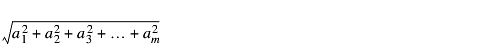
where a1, a2, and so on are the individual vector subcomponents within the selected component.
convert a Multi_Block object to an array of fields
mblock_to_fields extracts the array of fields contained in the Multi_Block object.
Multi_Block. The input multiblock dataset.
Mesh_Struct+Node_Data+Cell_Data_Struct. The array of fields extracted from multi_block.
create the mirror image of an unstructured Mesh
mirror generates a mesh that is the mirror image of the input mesh by reflecting the mesh about the X, Y, and/or Z plane. You can control each independently. Mirroring is useful for visualizing axisymmetric problems.
The input is any mesh. Any Node_Data that is present is ignored.
A port to connect to a user interface object that contains the macro's widgets. By default, it is connected to the default user interface object in the application in which the macro is instanced. (This default connection is not drawn.)
UItoggles. When on, its respective axis is mirrored. The default for all is on.
The output field is a reference to the input field, but with a new, modified xform transformation matrix object.
This is a renderable version of the output field.
Libraries.Examples.Visualization.Mirror_Scale
examples/mirr_scl.vData mappers that create Node_Data objects given data array(s)
The node_scalar and node_vector macros create Node_Data objects that can merge with a Mesh object to create a field. A Node_Data object represents the values of some dataset at the node points of a field, while the Mesh represents the locations of that field's nodes in space.
These macros simplify the process of generating field data by reducing the amount of data you must supply to create a field. Usually the output of one of these macros is combined, using combine_mesh_data, with the output of one of the mesh mapper macros to create a field.
array of any primitive type. Contains the node data to use. For node_scalar, the array's length should be the number of nodes in the dataset. For node_vector, the array's length should be nnodes * veclen.
Node_Data. The node data object containing the given data array.
Section 5.72, radius_data, rgb_data, argb_data, node_colors, node_normals, node_uv, node_uvw, pick_data [page 5-171]
deform a mesh by data vector at each node
offset "physically" deforms a mesh by the values of a one-, two-, or three-vector component located at each node. The first element of the vector translate's the node's X coordinate, the second (if present) translates the Y coordinate, and the third (if present) translates the Z coordinate. The magnitude of each translation is proportional to the values at the nodes multiplied by a scaling factor.
The input is any mesh with Node_Data. Its components can be a one-, two-, or three-element vector.
A port to connect to a user interface object that contains the macro's widgets. By default, it is connected to the default user interface object in the application in which the macro is instanced. (This default connection is not drawn.)
UIradioBoxLabel. Radio buttons to pick which component to use as the three-element vector that defines the offset. The default is the first (0th) component. If node data labels are present, they are displayed.
UIslider. A float slider used to scale the degree of distortion caused by the vector component. The default is 1.0. The range is -10.0 to 10.0.
The output is a new field containing as its mesh the original mesh distorted by the vector component times the scaling factor, and containing as its Node_Data a reference to the input Node_Data. A generic input Mesh creates a Mesh output. Mesh_Struct, Mesh_Unif, or Mesh_Rect input creates Mesh_Struct output.
This is a renderable version of the output field.
Libraries.Examples.Visualization.Offset
examples/offset.v
Libraries.Examples.Visualization.Surf_plot
examples/surf_plt.vproduce a slice of a structured field perpendicular to a coordinate axis
orthoslice subsets a structured field by extracting one slice plane. The slice plane can only be orthogonal to the X, Y, or Z axis.
The input must contain a structured mesh (mesh type Mesh_Struct, Mesh_Unif, or Mesh_Rect) and Node_Data. The input can be 1D, 2D, or 3D.
A port to connect to a user interface object that contains the macro's widgets. By default, it is connected to the default user interface object in the application in which the macro is instanced. (This default connection is not drawn.)
UIslider. An integer slider. Selects which axis (X = 0, Y = 1, Z = 2) the orthoslice is perpendicular to. The default is 0. If the field is 1D or 2D, three values are still displayed. Select the values meaningful for the input data.
UIslider. An integer slider. Selects which plane to extract from the input. The default is dims[axis]/2. The range is 0 to max_dim.
The output is a field with a new structured mesh of the same type as the input field. The mesh is the mesh of the slice. It contains the slice's Node_Data.
This is a renderable version of the output field.
Libraries.Examples.Visualization.Orthoslice
examples/orth.v
Libraries.Examples.Visualization.Null_Data
examples/nulldt.vsubset a volume using any number of 2D uniform grids as slicing planes
plane_crop subsets a field by outputting all whole cells that are inside or outside a volume created by an unlimited number of slice planes.
The input is a field with any Mesh. Node_Data is optional.
An array of Plane_Grids that will slice the volume. A Plane_Grid is defined as Grid_Unif+Space2+Dim2. It is, therefore, any 2D uniform grid.
A port to connect to a user interface object that contains the macro's widgets. By default, it is connected to the default user interface object in the application in which the macro is instanced. (This default connection is not drawn.)
UItoggle. When on, the entire cell intersected by a plane is output. If it is off, the entire cell is not output.
UItoggle. When on, the cells inside the slicing planes are output. If it is off, the cells outside the slicing planes are output.
The output is a new Mesh and Node_Data that is the plane-cropped input Mesh, plus any Node_Data for the output nodes. The mesh contains a reference to the input field's xform.
This is a renderable version of the output field.