5
Macros
This chapter provides an introduction and comprehensive reference material for the Data Visualization Kit high level macros.
- Note: Some of the macros described in this chapter are available only in the Developer Edition. Where this is the case, a line identifying this fact appears directly below the module name at the top of the page.
Visualization macros are macro objects that combine visualization base modules with UI objects in a structure that is convenient for building visualization networks and applications. Visualization macros have input/output ports and UI widgets that automatically appear on the Module Stack panel. You connect them using the Network Editor.
In Libraries.Main, the visualization macros are classified as follows:
- Modules and macros that input data files from disk or create data. Geometries, for example, create objects such as slice planes, 2D and 3D axes, crosshairs, arrows, and diamonds, that are used by other modules to slice data, represent vector quantities, act as data probes, show data, and so forth.
- Modules and macros that read data from disk are documented in this chapter.
- Geometries are documented in Chapter 4, Geometries".
- Modules and macros that primarily modify the field's Node_Data.
- Modules that primarily modify the field's mesh.
- Modules and macros that use the ip_Image data type for image processing. These are documented in Chapter 5, IP image processing macros".
- Modules and macros that render data on the screen. These objects are part of the Graphics Display Kit, not the Data Visualization Kit. They are documented in the Graphics Display Kit manual.
- Modules and macros that write data to disk files.
Visualization objects appear multiple times in a variety of places in the Libraries palette other than Main. To find them, use the Network Editor's Object Finder (see the User's Guide for details).
Most modules and macros report their status and their execution can be interrupted from the Module Stack Controls panel.
Most visualization modules and macros have sample networks that you can run showing how the object is properly connected within a network, and the kinds of effects it can produce on sample data.
Each reference page lists the sample networks that illustrate its use.
The examples are found in Libraries.Examples.Visualization in the Network Editor.
The reference pages for the modules include a path to the module. This path describes where you can locate the module in the network editor. Some modules belong to more than one library (for example, slice). To locate all paths to a particular module, use the Object Finder.
When determining which port on the icon corresponds to which documented item, remember that ports are documented from left to right. The first input port documented on the reference page is the leftmost port on the icon, the second input port documented is the second port from the left on the icon, and so on.
You can use a module or macro icon's Info panel to see the name and class of a port:
- With the cursor on the icon, press the right mouse button to activate the pulldown menu.
- Select Info. The first input port listed is the leftmost port on the icon, the second port listed is the second port from the left on the icon, and so on.
Visualization macros are defined in v/modules.v.
The Graphics Display Kit contains a GDmodes subobject called normals whose value specifies whether and how vertex normals are generated for Data Visualization Kit modules. The following table lists the allowed values for the normals subobject and their meanings:
GD_NORMALS_VERTEX is the default for most modules, and vertex normals are therefore generated.
However, for the following modules, the default setting is GD_NORMALS_NONE:
For more information on the GDmodes subobject, see Section 6.15, DefaultModes [page 6-51] in the Graphics Display Kit manual.
release massless particles into velocity field
advector releases a sample of zero mass particles into a field with a component that represents a velocity vector, for example, a fluid flow simulation. The particles have no initial direction or speed. The particles move through the velocity field according to the magnitude and direction of the vectors at the nodes in the volume. A forward differencing method is used to estimate the next position of each particle as a function of its current position and velocity (see the section labelled Algorithm on page 5-10).
Advection starts when you turn the Run toggle on. Advection for individual particles stops when one of the following conditions occurs:
- A particle exceeds the Max Segments value.
- The particle's velocity drops below the Min Velocity.
- The particle goes outside the field's bounds.
Advection of all particles stops when one of the following two conditions occurs:
- The input is any mesh with Node_Data. The first component is used and must be a scalar or a two- or three-element velocity vector. You can use extract_component before this macro to get the component you want out of a multi-component field.
- Any mesh whose coordinates represent the sample points. Meshes that are not unstructured are accepted, but a local unstructured version is generated during execution.
- To create this sampling mesh you could use the plane object in Geometries.FPlane or the slice macro.
- A Grid describing a glyph to represent the particles. This is simply a mesh describing the geometry of the glyph. Any mesh can be used (for example, that of a teapot), but for convenience you can use the Geometries objects to generate arrows or solid arrows, and so on
- A port to connect to a user interface object that contains the macro's widgets. By default, it is connected to the default user interface object in the application in which the macro is instanced. (This default connection is not drawn.)
- UIradioBoxLabel. A radio box to pick which of the input field's components to use as the velocity vector. The selection can be a one-, two-, or three-element vector. The default is the first (0th) component. If node data labels are present, they are displayed.
- UIslider. An integer slider that sets the number of integration steps used within one grid "cell" to compute the streamline/particle path. The default is 2. The range is from 0 to 16.
- UIslider. An integer slider that sets the total number of integration steps. When an individual particle exceeds this value, integration for it stops. The range is from 1 to 10000. The default is 256.
- UIslider. An integer slider that sets the order of integration. Higher orders are more accurate, but execute more slowly. The default is 2. The range is from 1 to 4.
- UIslider. A float slider. When a particle falls below this velocity, the integration process for that particle stops. The default is 0.00001. The range is from 0.0 to unbounded. You can use this to prevent wasted computation for particles barely moving, or even stationary (Min Velocity = 0).
- UIradioBoxLabel. A radio box that controls whether particles are advected forward or backward from the starting sample points. The default is forward.
- UIradioBoxLabel. A radio box that establishes how glyphs are rendered to represent the data values. (Glyphs are always colored by the magnitude of the data values in the component.) The choices are scalar, vector, or components:
Scale the glyph by the magnitude of the vector at that position. Also rotate the glyph in X, Y, (and Z) by the first, second, (and third) vector subcomponent values at that position. For example, a Cross3D in_probe would be rotated to reflect the vector values.
Scale the glyph in X, Y, (and Z) by the first, second, (and third) vector subcomponent values at that position. For example, a Cross3D in_probe's three lines would be individually scaled to match the vector values.
- UItoggle. If off, the sizes of the glyphs are proportional to the data component values at each node. If on, all glyphs are the same size. The default is off.
- UIslider. A float slider to adjust the sizes of the glyphs. The default is 1.00. The range is 0.0 to 100.00.
- UIslider. A float. The time value along the original streamline continuum at which to start advection. (See DVadvect man page.) The default is 0.0.
- UIslider. A float. The time value along the original streamline at which to halt advection of all particles. The default is 1.0.
- UIslider. A float. The value by which to increment the time along the original streamline continuum for each advection step. The default is 0.2.
- UIfieldTypein. An output only widget that displays the current time in the count from Start Time to End Time.
- UItoggle. Starts or stops advection.
- UItoggle. Reset Time to the value of Start Time.
- UItoggle. When End Time is reached, start the advection again at Start Time.
- The output is a new unstructured Mesh composed of the original mesh plus the meshes representing the particles. Its new Node_Data element's values represent the selected velocity component.
- This output field is a new unstructured mesh of cell type Polyline that represents the streamlines. Its new Node_Data contains the selected element's velocity component. The output also contains a reference to the input field's xform.
- This is a renderable version of the out_fld output field.
- This is a renderable version of the out_fld1 output field.
advector uses precomputed streamlines (from DVstream) as particle paths. It integrates velocity along the streamlines to calculate the new position of the particles at each time step.
The streamlines are originally calculated using the Runge-Kutta method of specified order with adaptive time steps.
Libraries.Examples.Visualization.Advect
examples/advect.vrelease massless particles into Multi_Block velocity field
advect_multi_block releases a sample of zero mass particles into a field with a component that represents a velocity vector, for example, a fluid flow simulation. The particles move through the velocity field according to the magnitude and direction of the vectors at the nodes in the volume. A forward differencing method estimates the next position of each particle as a function of its current position and velocity (see "Algorithm" on page 5-15).
Advection starts when you turn the Run toggle on. Advection for an individual particle stops when one of the following conditions occurs:
- The particle exceeds the Max Segments value.
- The particle's velocity drops below the Min Velocity.
- The particle goes outside the field's bounds.
Advection of all particles stops when one of the following conditions occurs:
- The input is a Multi_Block object. A Multi_Block object can be created with fields_to_mblock or Plot3D_Multi_Block. A Multi_Block object consists of an array of fields describing the data and some ancillary metadata. The first component of the fields' data is used and must be a scalar or a two- or three-element velocity vector. You can use mblock_to_fields, extract_component_ARR and fields_to_mblock before this macro to get the component you want from a multi-component Multi_Block.
- Any mesh whose coordinates represent the sample points. Meshes that are not unstructured are accepted, but a local unstructured version is generated during execution.
- To create this sampling mesh you could use the slice macro or the plane object in Geometries.FPlane.
- A Grid describing a glyph to represent the particles. This is simply a mesh describing the geometry of the glyph. Any mesh can be used (for example, that of a teapot) but for convenience you can use the Geometries objects to generate arrows or solid arrows, and so on
- A port to connect to a user interface object that contains the macro's widgets. By default, it is connected to the default user interface object in the application in which the macro is instanced. (This default connection is not drawn.)
- UIslider. An integer slider that sets the number of integration steps used within one grid "cell" to compute the streamline/particle path. The default is 2. The range is from 0 to 16.
- UIslider. An integer slider that sets the total number of integration steps. When an individual particle exceeds this value, integration for it stops. The range is from 1 to 10000. The default is 256.
- UIslider. An integer slider that sets the order of integration. Higher orders are more accurate, but execute more slowly. The default is 2. The range is from 1 to 4.
- UIslider. A float slider. When a particle falls below this velocity, the integration process for that particle stops. The default is 0.00001. The range is from 0.0 to unbounded. You can use this to prevent wasted computation for particles barely moving, or even stationary (Min Velocity = 0).
- UIradioBoxLabel. A radio box that controls whether particles are advected forward (1) or backward (0) from the starting sample points. The default is forward.
- UIradioBoxLabel. A radio box that establishes how glyphs are rendered to represent the data values. (Glyphs are always colored by the magnitude of the data values in the component.) The choices are:
Scale the glyph by the magnitude of the vector at that position. Also rotate the glyph in X, Y, (and Z) by the first, second, (and third) vector subcomponent values at that position. For example, a Cross3D in_probe would be rotated to reflect the vector values.
Scale the glyph in X, Y, (and Z) by the first, second, (and third) vector subcomponent values at that position. For example, a Cross3D in_probe's three lines would be individually scaled to match the vector values.
- UItoggle. If off (0), the sizes of the glyphs are made proportional to the data component values at each node. If on (1), all glyphs are the same size. The default is off.
- UIslider. A float slider to adjust the sizes of the glyphs. The default is 1.00. The range is 0.00 to 100.00.
- UIslider. The time value along the original streamline continuum at which to start advection. (See DVadvect reference page.) The default is 0.0.
- UIslider. The time value along the original streamline continuum at which to halt advection of all particles. The default is 1.0.
- UIslider. The value by which to increment the time along the original streamline continuum for each advection step. The default is 0.2
- UIfieldTypein. An output only widget that displays the current time in the count from Start Time to End Time.
- UItoggle. Starts (1) or stops (0) advection.
- UItoggle. Reset Time to the value of Start Time.
- UItoggle. When End Time is reached, start the advection again at Start Time.
- The output is a new unstructured Mesh composed of the original mesh plus the meshes representing the particles. Its new Node_Data element's values represent the selected velocity component.
- This output field is a new unstructured mesh of cell type Polyline that represents the streamlines. Its new Node_Data contains the selected element's velocity component. The output also contains a reference to the input field's xform.
- This is a renderable version of the out_fld output field.
- This is a renderable version of the out_fld1 output field.
advect_multi_block uses precomputed streamlines (from DVstream) as particle paths. It integrates velocity along the streamlines to calculate the new position of the particles at each time step.
The streamlines are originally calculated using the Runge-Kutta method of specified order with adaptive time steps.
generate a bounding box of a 3D structured field
bounds generates lines and/or surfaces that indicate the bounding box of a 3D structured field. This is useful when you need to see the shape of an object and the structure of its mesh. For example, isosurface can produce a fairly cryptic shape floating without context in space, but when combined with bounds, you see the isosurface within its surrounding mesh.
- The input field must contain any type of structured mesh (mesh type Mesh_Struct, Mesh_Unif or Mesh_Rect). Node_Data can be present, but is only used if you switch on Data.
- A port to connect to a user interface object that contains the macro's widgets. By default, it is connected to the default user interface object in the application in which the macro is instanced. (This default connection is not drawn.)
- UIradioBoxLabel. Selects which of the input field's components to send to the output, if Data is also turned on. The default is the first (0th) component. If node data labels are present, they are displayed.
- UItoggle. When on, draws a wireframe around the perimeter extents of the mesh. The default is on.
- UItoggle. When on, causes the Imin/Imax, Jmin/Jmax, Kmin/Kmax controls to produce a wireframe representation of the mesh grid at that plane. The default is off.
- UItoggle. When on, causes the Imin/Imax, Jmin/Jmax, Kmin/Kmax controls to produce a solid face representing the location of that plane extent. The default is off.
- UItoggle. When on, each of these switches displays the grid (Edges turned on) or plane (Faces turned on) on one of the six faces of the hull. Imin/Imax draw a mesh or face showing the 2D slice of field objects with the minimum/maximum index value in the first dimension. Jmin/Jmax draw a mesh or face showing the 2D slice of field objects with the minimum/maximum index in the second dimension. Kmin/Kmax control the third dimension. The default for all is off.
- UItoggle. When on, makes bounds copy the selected component's Node_Data values at node points along the output mesh to the output field. Because the data is present, the bounds lines can be colored by the interpolated data values of the selected Node_Data component. Otherwise, the lines display as white in the renderer. The default is off.
- The output field contains a new unstructured Mesh object with cell type Polyline (Edges selected) and/or Quad (Faces set) representing the bounds. If Data was selected, the output field also contains a Node_Data that is the selected component's values at nodes on the output mesh.
- This is a renderable version of the output field.
Libraries.Examples.Vizualization.Crop
examples/crop.vproduce a Point mesh representing geometric centers of each cells
cell_centers module produces a mesh containing Point cell set, each point of which represents a geometrical center of a corresponding cell in the input mesh. The coordinates of cell centers are calculated by averaging coordinates of all the nodes of a cell. The number of nodes in the output mesh is equal to number of cells in the input mesh. If the input mesh contains Cell_Data it becomes a Node_Data in the output mesh with each node values equal to corresponding cell value. You can use this module to create a position mesh for the glyph module (see Section 5.45, glyph [page 5-105]).
- The input must contain any type of mesh.
- The output field contains a new mesh that consists of points representing geometrical centers of a corresponding cells in the input mesh.geoetric centers. It also may contain a Node_Data that corresponds to Cell_Data in the input mesh.
- This is a renderable version of the output field.
Libraries.Examples.Visualization.Cylinder_Plot_Unif
examples/cyl_plot_unif.vperform arbitrary math operations on cell-based data
cell_data_math performs arbitrary math operations on up to four cell-based datasets. You can use any operation or expression that can be specified in the V language to operate on the data. The expression you enter may use #1, #2, #3, and #4 to stand for the four input fields.
- Mesh+Cell_Data. Input to math expression. Use "#1" in the expression to refer to this field.
- Mesh+Cell_Data. Input to math expression. Use "#2" in the expression to refer to this field.
- Mesh+Cell_Data. Input to math expression. Use "#3" in the expression to refer to this field.
- Mesh+Cell_Data. Input to math expression. Use "#4" in the expression to refer to this field.
- A port to connect to a user interface object that contains the macro's widgets. By default, it is connected to the default user interface object in the application in which the macro is instanced. (This default connection is not drawn.)
- UItext. Math expression to perform on the cell data of the inputs. All V language expressions are valid; use #1 through #4 to refer to the input fields. For example, the expression sqrt(#1 * 10 + sin(#2/#3))computes a function of the first three inputs.
- Mesh+Cell_Data. Contains the result of applying the given expression to the input field(s).
- Renderable object. Renderable version of out_fld.
convert Cell_Data to Node_Data
cell_to_node converts Cell_Data to Node_Data. It is necessary to convert cell-based data to node data when the visualization modules or macros selected do not process cell-based data.
- Note: All nodes referenced by a cell with a NULL value will have their Node_Data set to NULL.
- The input is a field with an unstructured Mesh and Cell_Data.
- A port to connect to a user interface object that contains the macro's widgets. By default, it is connected to the default user interface object in the application in which the macro is instanced. (This default connection is not drawn.)
- UIoptionBoxLabel. A series of buttons that let you select which components in the input field to convert to Node_Data. You can select multiple components. If the Cell_Data contains multiple cell_sets, the conversion is performed on the specified components in each cell_set.
- UIslider. An integer that sets the order of interpolation. Allowed values are:
A node's value is computed by interpolating values using distances from the node to the adjoining cell centroids.
- The output is a reference to a merged object that contains the new Node_Data, plus the existing Mesh and Cell_Data.
- This is a renderable version of the output field.
Libraries.Examples.Visualization.Cell_Data
examples/celld.vcreate plot of blocks based on the height (value) of a 2D field
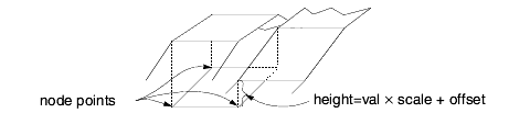
city_plot creates a block on each node of the input mesh. The color and height (out of the grid) of the block are determined independently by selectable input data components at that node. The lower left (min X and Y) corner of the block is at the node's coordinate, so the city plot extends over the dimensions of the field by one block width (in X) and length (in Y), because the block at (maxX, maxY) extends from that point to (max_x + scale_x * x spacing, max _y + scale_y * y spacing).
- Mesh_Unif + Node_Data + Dim2. The 2D field to be plotted.
- A port to connect to a user interface object that contains the macro's widgets. By default, it is connected to the default user interface object in the application in which the macro is instanced. (This default connection is not drawn.)
- UIradioBoxLabel. Selects which component of the input to map to the height of the block at that point of the grid.
- UIradioBoxLabel. Selects which component of the input to map to the color of the block at that point of the grid.
- UItoggle. When turned on (1), the heights of the blocks are normalized to a constant value set by the height scale, and the glyph_comp is ignored.
- UIslider. Scales the input height value by this amount. If normalize is on, this value becomes the height of the blocks. Height is measured in the coordinate system of the input field.
- UIslider. Scales the X size of each block relative to the size of that block's cell width. scale_x of 1 means the block takes up the full width of the cell and abuts the next block (in X); scale_x of 0.5 means the block takes up 1/2 the width of the cell.
- UIslider. Scales the Y size of each block relative to the size of that block's cell width. scale_y of 1 means the block takes up the full length of the cell and abuts the next block (in Y); scale_y of 0.5 means the block takes up 1/2 the length of the cell.
- The output field is an unstructured Mesh of cell type Quad containing the blocks.
- Renderable object corresponding to out_fld.
Libraries.Examples.Visualization.City_Plot
examples/city_plot.vclamp minimum and maximum values of data
clamp transforms the values of the selected field component subcomponent as follows:
- If Above max_value is set, any value above max value is set to max value.
- If Below min_value is set, any value below min value is set to min value.
- Otherwise, the values are not changed.
If Above max_value and Below min_value are on, the output field's selected component values are all in the range of min value <= value <= max value. Null data values are not affected.
Note the difference between clamp and the threshold macro:
- threshold sets values outside the range to a specified null value.
- clamp sets values outside the range to min value and/or max value.
- The input field must contain a Node_Data object. If a Mesh is present, it is passed along untouched as a reference in the output field. The field's data components can be scalar or vector.
- A port to connect to a user interface object that contains the macro's widgets. By default, it is connected to the default user interface object in the application in which the macro is instanced. (This default connection is not drawn.)
- UIradioBoxLabel. Selects which of the input field's components to clamp. The default is the first (0th) component. If node data labels are present, they are displayed.
- UIslider. If the selected data component is non-scalar, you can pick which subcomponent to clamp. The range is 0 (first subcomponent) to the number of subcomponents. The default is 0.
- UItoggle. When on, clamps data above the max value. The default is off.
- UItoggle. When on, clamps data below the min value. The default is on.
- UItoggle. When on, clamp recalculates the data's minimum and maximum values. The default is off.
- UIslider. Double precision floating point sliders that set the min and max values. The default is set to the input field component's node data minimum and maximum. The range shown is from the component's node data minimum to its maximum. The double precision value is converted to the data type of the input field before use. Two decimal points of precision are given.
- The output field contains a new Node_Data object that is the clamped component. If a Mesh was present, the output field contains a reference to that mesh.
- If a Mesh was present, this is a renderable version of the output field. Otherwise, rendering objects generate an error.
Libraries.Examples.Vizualization.Clamp
examples/clamp.vtake components from two different fields to make a new n-component field
combine_comp takes the selected components from the first input field, and the selected components from the second input field, creating a new output field with n components. The output field's mesh, if present, comes from the first input field. For example, selecting the second components from each of the fields (a, b, c) and (d, [e, f, g]) results in the field (b, [e, f, g]).
- This input field must contain any mesh with Node_Data object. If a mesh is present, it is passed along untouched as a reference in the output field. The field's data components can be scalar or vector.
- This input field must contain a Node_Data.
- A port to connect to a user interface object that contains the macro's widgets. By default, it is connected to the default user interface object in the application in which the macro is instanced. (This default connection is not drawn.)
- UIoptionBoxLabel. Select which of the input fields' components to combine. The default for both is the first (0th) component. If node data labels are present, they are displayed.
- The output field is a Node_Data that is an array of references to the two selected Node_Data components. If a mesh was present, the output field contains a reference to that mesh.
- This is a renderable version of the output field.
combines a mesh and cell data array to produce a field
combine_mesh_cell_data combines a mesh and and a cell data array. The in_data object represents the values of some dataset at the cells of a field, while the in_mesh represents the locations and connectivity of that mesh's nodes and cells. The in_mesh object should have one cell set to which cell data is added. The in_data can be a primitive array of any type: byte, int, float, etc. If in_data is a one dimensional array, the scalar cell data is created. The dimension of this array should be the same as ncells in in_mesh. If it is two-dimensional array, the low dimension is used for data veclen and the high dimension should be the same as ncells in in_mesh.
This macro simplifies the process of generating field; it is used to combine the output of a mesh mapper with the raw array of cell data.
- Mesh containing one cell set.
- prim. This array can be of any primitive type (int, float. etc.)
- Mesh+Cell_Data. Mesh with cell data.
- Output renderable object corresponding to out.
combine a mesh and some node data to produce a field
combine_mesh_data combines a mesh and some node data. A Node_Data object represents the values of some dataset at the node points of a field, while the Mesh represents the locations of that field's nodes in space.
This macro simplifies the process of generating field data by reducing the amount of data you must supply to create a field. Usually this macro is used to combine the output of a mesh mapper with the output of one or more data mappers.
- Mesh. This input is the Mesh part of the result.
- Node_Data. This input is the Node_Data part of the result.
- Mesh+Node_Data. This contains the two inputs, merged.
- Output renderable object corresponding to out.
Section 5.72, radius_data, rgb_data, argb_data, node_colors, node_normals, node_uv, node_uvw, pick_data [page 5-171]
combine different Node_Datas into one Node_Data with multiple components
combine_node_datas combines several sets of node data (for example, radius and color data), into one node dataset that can be incorporated into a field. It makes each node_data into a component of the output Node_Data. If an input has more than one component, all its components are inserted into the output in order, at the same level as the other components from other inputs.
A Node_Data object represents the values of some dataset at the node points of a field, while the Mesh represents the locations of that field's nodes in space.
These macros simplify the process of generating field data by reducing the amount of data you must supply to create a field. Usually the output of one of these macros is combined, using combine_mesh_data, with the output of one of the mesh mapper macros to create a field.
- Node_Data[]. This input is an array of Node_Data objects. Each one becomes one or more components of the output Node_Data.
- Node_Data. This contains all the components from the inputs.
Section 5.72, radius_data, rgb_data, argb_data, node_colors, node_normals, node_uv, node_uvw, pick_data [page 5-171]
combine three scalars into an RGB image
combine_rgb combines three scalar 2D, 2-space byte input fields into an RGB image. This macro is similar to combine_vect except it only works on exactly three 2D 2-space uniform byte fields, and it sets the resulting node data ID to tell the renderer that it is an RGB image.
- Mesh_Unif+Dim2+Byte+Space2+Node_Data. This field represents the red channel of the image.
- Mesh_Unif+Dim2+Byte+Space2+Node_Data. This field represents the green channel of the image.
- Mesh_Unif+Dim2+Byte+Space2+Node_Data. This field represents the blue channel of the image.
- RGB image field.
- Renderable object corresponding to out_fld.
combine n scalar components into a single n-vector component
combine_vect takes all the selected data components, which must be scalar, and produces a single output data component that is the specified veclen long. For example, selecting the first and third components of (a, b, c, [e,f,g]) results in the field ([a, c]).
- The input field must contain a Node_Data object. If a mesh is present, it is passed along untouched as a reference in the output field. The field's data components must include at least two scalar components.
- A port to connect to a user interface object that contains the macro's widgets. By default, it is connected to the default user interface object in the application in which the macro is instanced. (This default connection is not drawn.)
- UIslider. Sets the number of scalar components to combine and the out_fld's single component veclen. The default is 3. The range is 1 to 4.
- UIoptionBoxLabel. Selects which of the input field's components to combine. If you select vector components, only the first vector subcomponent is extracted. If node data labels are present, they are displayed. The default is the first three components.
- The output field contains a new Node_Data that is a data array of references to the selected components in the original input Node_Data. It has one component with veclen equal to the specified veclen. If a mesh was present, the output field contains a reference to that mesh.
- If a mesh was present, this is a renderable version of the output field. Otherwise, rendering objects generate an error.
Libraries.Examples.Visualization.Advect
examples/advect.v
Libraries.Examples.Visualization.Curl
examples/curl.v
Libraries.Examples.Visualization.Glyph_Interp
examples/glh_intp.vconcatenate elements of several arrays or individual scalar primitives into an array
These modules concatenate elements of several arrays or individual scalar primitives into an output array. Input arrays may have any dimensionality, but are treated as 1-dimensional, in memory order.
Input arrays can have different total sizes; the size of the output array is the sum of the sizes of the input arrays. The output array contains all elements from the first array, followed by all elements from the second array, and so on.
For example, this can be used to create an XYZ coordinate array from separate X, Y, and Z arrays.
- prim[]. One of the input arrays or scalar primitives.
- prim[]. One of the input arrays or scalar primitives.
- prim[]. One of the input arrays or scalar primitives.
- prim[]. One of the input arrays or scalar primitives.
- prim[]. The output array containing the concatenated data.
create an isovolume bounded by two isosurfaces (3D) or isolines (2D)
contour creates a field that is the volume bounded by two isosurfaces (if the field is 3D) or two isolines (if the field is 2D).
For example, you could set the min level and max level isosurfaces to densities found just outside a bone. When combined, the isovolume produced would be the bone itself.
The isosurfaces or isolines are colored by the first map component selected. All of the selected map components are in the Node_Data of the output field.
- Note: The contour module does not generate vertex normals by default. For more details, see Section 5.1.8, Vertex normal generation [page 5-4].
- The input is any mesh with Node_Data. A 2D mesh will produce isolines. A 3D mesh produces isosurfaces. At least one of the components must be scalar.
- A port to connect to a user interface object that contains the macro's widgets. By default, it is connected to the default user interface object in the application in which the macro is instanced. (This default connection is not drawn.)
- UIradioBoxLabel to pick which component to isosurface/isoline. The selected component must be scalar or the message "iso: first component is not scalar" is written to stderr. The default is the first (0th) component. If node data labels are present, they are displayed.
- UIoptionBoxLabel to pick components that will be written to the output field. In addition, the first selected component will be mapped onto the isosurface/isoline (for example, map pressure value onto a density isosurface). The selection does not have to be scalar. The default is the first (0th) component. If node data labels are present, they are displayed. Where the isosurface/isoline does not exactly intersect a node, the data value is linearly interpolated based on the surface's distance from the adjacent nodes.
- UIslider. Float sliders that set the minimum and maximum isosurface/isoline values, between which data is extracted. The default is 0.0. The range is from the minimum data value in the selected contour component to the maximum data value in the selected contour component. The data type of the slider is converted to the data type of the node data before use.
- The output field is an unstructured Mesh of cell type Tri (3D) or Line (2D) that represents the contour volume. Its Node_Data is the values within the volume. The surface values are interpolated along the isosurface/lines.
- This is a renderable version of the output field.
contour uses the Marching Cubes algorithm to construct the isosurfaces/isolines. See W. Lorensen and H. Cline, "Marching Cubes: A High Resolution Surface Reconstruction Algorithm." Computer Graphics 21(4) (SIGGRAPH Proceedings, 1987), July, 1987, pp. 163-169.
This algorithm has a known limitation. There are cases where there are two possible paths that the isosurface could take through a cell, and only one is the correct path. If isosurface picks the wrong path, a discontinuity appears as a hole in the surface.
Libraries.Examples.Vizualization.Contour
examples/cont.v
Libraries.Examples.Vizualization.Contour_2D_Unif
examples/cont2uni.v
Libraries.Examples.Vizualization.Cylinder
examples/cyl.vcopy a mesh to a selected region of an output array of meshes
copy_ROI copies an input mesh, typically created by one of the Graphics Display Kit's interactive drawing modules (for example, ClickSketch, ContinuousSketch) to an array of output meshes. This module is a quick way to create an array of ROIs that correspond to a volume. The ROIs can subsequently be edited individually by using the EditMesh module.
The size of the output mesh array is determined by using a reference input field. The input mesh may be copied to a region of the output mesh array by using the start and stop parameters appropriately.
- The reference input field must be uniform, 3D and have node data. This field is used to dimension the output array of meshes
- The input mesh to be copied into the output mesh array.
- UIfieldTypein. Start index into the output mesh array.
- UIfieldTypein. Start index into the output mesh array.
- UItoggle. When set, Run starts the copy operation. It is automatically cleared when the copy operation is completed.
- The output array of meshes. This array is dimensioned by the reference input field. Depending on the values of Start and Stop, all or part of the output
Libraries.Examples.Visualization.Tile_ROI
Libraries.Examples.Visualization.Display_Vol_ROIextract a subset of a structured field
crop reduces the size of a structured field by extracting the data within a specified range of its dimensions. The process is analogous to "cropping" a photographic image. Typical uses are to eliminate uninteresting portions of the data and to increase processing speed by reducing the amount of data.
- The input must contain a structured mesh object (Mesh_Struct, Mesh_Rect, or Mesh_Unif), and a Node_Data object. The mesh can be 1D, 2D, or 3D.
- A port to connect to a user interface object that contains the macro's widgets. By default, it is connected to the default user interface object in the application in which the macro is instanced. (This default connection is not drawn.)
- UIsliders. Used to set crop dimensions. I min, J min, and K min set the lower bound array index in their respective dimensions; I max, J max, and K max set the upper bound array index in their respective dimensions. All default to 0 (min) and the maximum dimension of the mesh (max), so that the default is no cropping. Their range is from 0 to the maximum dimension of the Mesh for I, J, and K. All three pairs of controls appear no matter what the dimensionality of the input Mesh. Use just the controls meaningful for the input data.
- The output field contains a new Mesh_Struct and a new Node_Data associated with the cropped region.
- If the input was a Mesh_Rect or a Mesh_Unif, its points array (extents) are modified to retain the mesh's position in space.
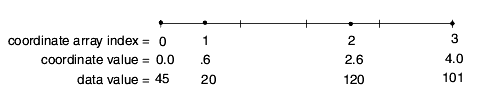
- For example, the following 1D field has a points array (extents) from 0 to 49.
- You crop the field using an I min of 30 and an I max of 49. The output field has coordinate indices from 0 to 19 and a points array from 30 to 49.
- The output field also contains a new Node_Data that has the data within the cropped region.
- This is a renderable version of the output field.
Libraries.Examples.Vizualization.Crop
examples/crop.vcompute the curl of a vector field
curl computes the curl of a vector field with any mesh type.
- The input must be a field with any type of mesh and Node_Data. At least one of the Node_Data's components must be a three-element vector.
- A port to connect to a user interface object that contains the macro's widgets. By default, it is connected to the default user interface object in the application in which the macro is instanced. (This default connection is not drawn.)
- UIradioBoxLabel. A radio box to pick which component of in_field to use to compute the curl. You must pick a three-element vector component. The default is the first (0th) component. If node data labels are present, they are displayed.
- The output field contains a new Node_Data that has a three-element float at each node representing the curl. Its mesh is a reference to the input mesh.
- This is a renderable version of the output field.
The algorithm used to compute the curl in structured meshes is a finite difference approximation based on a central difference scheme. For unstructured meshes, the function is based on the cell shape functions and their derivatives.
In both cases, where the input is the vector function:

The equation used to compute the curl is:

Libraries.Examples.Vizualization.Curl
examples/curl.vcut off a portion of a field on one side of cutting plane
cut lets you cut (divide) a field into two pieces, and output one of the pieces. You position an arbitrarily-oriented cutting plane within the field, and select which side of the cutting plane you wish to output. Output is generated every time the cutting plane moves.
- Note: The cut module does not generate vertex normals by default. For more details, see Section 5.1.8, Vertex normal generation [page 5-4].
- The input must be a field with any type of 2D or 3D mesh and any type. It may optionaly have node and/or cell data components
- The cutting plane. This is generated by the plane object found in Geometries.FPlane. The plane object has its own Plane Transformation panel that controls plane rotation, translation, and scale, as well as controls to specify its size when it is connected to the default user interface object in the application in which the macro is instanced.
- A port to connect to a user interface object that contains the macro's widgets. By default, it is connected to the default user interface object in the application in which the macro is instanced. (This default connection is not drawn.)
- UIoptionBox. A selection to pick which components of in_field's node data (if prsent) to send to the output field. You can pick more than one or none. The default is the first (0th) component. If node data labels are present, they are displayed.
- UIoptionBox. A selection to pick which components of in_field's cell data (if present) to send to the output field. You can pick more than one or none. The default is the first (0th) component. If cell data labels are present, they are displayed.
- UItoggle. Picks which side of the slice plane to send to the output field. The default is on.
- UIslider. A float slider that moves the plane through the field perpendicular to the plane. Though the Plane Transformation panel has X, Y, and Z transformation controls, it is usually easier to use plane's controls to orient and size the plane, but use this plane distance control to move the plane. cut generates output whenever the slice plane moves. The default distance is 0.0 and the range is the extents of the field.
- The output field contains a new mesh object that is the subset of the original mesh. It has the same type as the input mesh. It may have node and/or cell data containing the selected components. Its extents are set to retain the position of the cut section of the field in space.
- This is a renderable version of the output field.
Libraries.Examples.Vizualization.Cut
examples/cut.vmacro that includes cut and cutting plane
cut_plane is a macro that includes the cut macro and an FPlane cutting plane object. It cuts away the part of a field above or below the arbitrarily-oriented cutting plane, revealing the internal structure.
- Note: The cut_plane module does not generate vertex normals by default. For more details, see Section 5.1.8, Vertex normal generation [page 5-4].
- The input field to cut. You can specify any 2D or 3D mesh with any primitive type of node data and/or cell data.
- A port to connect to a user interface object that contains the macro's widgets. By default, it is connected to the default user interface object in the application in which the macro is instanced. (This default connection is not drawn.)
- int[]: UIoptionBoxLabel. Select which node data component(s) are to be mapped onto the resulting mesh
- int[]: UIoptionBoxLabel. Select which cell data component(s) are to mapped onto the resulting mesh.
- UItoggle. Selects whether the part of the mesh above (1) or below (0) the cutting plane is removed. Above is in the positive Z direction of the cutting plane.
- UIslider. The plane at which the field is cut can be offset from the plane described by the internal plane object, which is what is transformed by the Plane Transform Editor. The offset is in the direction of the Z axis of the cutting plane. Note that if you offset the cutting plane from the plane object, the plane object output still shows the position of the plane object, not the actual cutting plane.
- UIbutton. This button brings up the plane transform editor panel, which you can use to transform the cutting plane to any arbitrary orientation.
- Mesh[+Node_Data] [+Cell_Data]. The mesh with the part above or below the cutting plane removed. It may have node and/or cell data from the part of the input field.
- Plane_Mesh. A mesh containing the cutting plane. This is simply a rectangle spanning the minimum and maximum of the first two dimensions of the field. It is transformed to lie at the correct spatial location.
- Renderable object corresponding to out_fld.
- Renderable object corresponding to out_plane.
show 3D uniform field as a texture-mapped sliced solid
cut_texture3D shows a 3D uniform field as a solid, with one slice cut off to reveal the interior structure. The slice plane can be moved through the volume perpendicular to the X, Y, and Z axes. Output is generated every time the slice plane moves.
cut_texture3D differs from interp_texture3D in the following ways:
- Its slicing plane can only be moved orthogonal to the X axis.
- It can display the exterior surfaces of the volume.
Texture mapping is much faster than the sampling techniques used by DVslice, particularly for large datasets. The point sampling done by the texture mapping technique is always done at the resolution of the data; thus, differences in data values within a small area are not obscured, as they can be with DVslice.
- The input must be a field with a Mesh_Unif, Space3, Dim3, and Node_Data.
- The slicing plane. This is generated by the Plane object found in Geometries.Plane or Geometries.FPlane. The plane object has its own Plane Transformation panel that controls plane rotation, translation, and scale, as well as controls to specify its size when it is connected to the default user interface object in the application in which the macro is instanced.
- A colormap to provide the texture map. From Libraries.Main.Fields.Data.colormap.
- A port to connect to a user interface object that contains the macro's widgets. By default, it is connected to the default user interface object in the application in which the macro is instanced. (This default connection is not drawn.)
- UIoptionBoxLabel. An option box to pick which components of in_field to texture map. You can pick more than one. The components must be scalar. The default is the first (0th) component. If node data labels are present, they are displayed.
- UItoggle. Picks which side of the slice plane to send to the output field.
- UIslider. A float slider that moves the plane through the field perpendicular to the plane. Though the Plane Transformation panel has X, Y, and Z transformation controls, it is usually easier to use plane's controls to orient and size the plane, but use this plane distance control to move the plane. cut_texture_3D generates output whenever the slice plane moves. The default distance is 0.0 and the range is the extents of the field.
- The output field contains a new mesh object that is the subset of the original mesh. It has the same type as the input mesh. It has a new Node_Data containing the texture mapping u, v, w values. Its points array (extents) is set to retain the position of the volume of the field in space.
- This is a renderable version of the output field.
cut_texture3D creates its picture of the volume data using 3D texture mapping. In this method, the boundary of the volume has three values, u, v, w, associated with each of its vertices. Where the slice planes intersect this volume, u, v, w values are computed for the vertices of the resulting solid. These values are attached to the vertices of the output object. Viewers use the u, v, w information to create the texture-mapped rendering.
Libraries.Examples.Vizualization.Cut_Texture
examples/cut_txt.vproduce a set of cylindrical glyphs that allow you to visualize two dimensional table data
cylinder_plot_unif allows you to visualize two dimensional node data that can be thought of as a table having some number of columns and rows. Each column in the table is represented with a cylinder glyph. A cylinder is divided in either vertical or angular direction into a number of segments equal to the number of rows in the column. Each segment is scaled (in either vertical or angular direction) proportionally to the data value of the row. The height or radius of each cylinder can optionally be scaled by the total value of the column (sum of all rows). The sides of the cylinder can optionally be colored by the total column value.The resultant image looks like a 3D pie chart.
- The input must contain a 2-dimensional uniform mesh (Mesh_Unif+Dim2) plus Node_Data.
- This port is optional. It is a grid describing the location of the cylinders. If nothing is connected to this port, the module will use coordinates of in_field to position the cylinders. This port is useful, for example, to position a cylindrical glyph at certain locations on a map.
- A port to connect to a user interface object that contains the macro's widgets. By default, it is connected to the default user interface object in the application in which the macro is instanced. This default connection is not drawn.
- UIradioBoxLabel. Radio buttons to pick which input Node_Data component to use to create cylinders. The default is the first (0th) component.
- UItoggle. Indicates whether to use angular of vertical segmentation for each cylinder. The default is off (angular segmentation).
- UItoggle. Indicates whether a height for each cylinder (representing a column of an input table data) is scaled by the total value of the column (sum of all rows).
- UItoggle. Indicates whether a radius for each cylinder (representing a column of an input table data) is scaled by the total value of the column (sum of all rows).
- UItoggle. Indicates whether the sides of each cylinder (representing a column of an input table data) are colored by the total value of the column (sum of all rows).
- UIfield. Represents a default radius value for all cylinders. If "scale radius by total" is set to on, this value is used as the scale for radii of the cylinders.
- UIfield. Represents a scale value for heights for the cylinders. If "scale height by total" is set to off, this value is used as the height for all the cylinders.
- UIslider. An integer value that represents the total number of sub-divisions for each cylinder. This number is used to control the graphical accuracy of the cylinders shape - the higher the value, the more accurate the cylinder is drawn (with a corresponding increase in drawing time). If this value is set to 4 you will get rectangular (4-sided) blocks instead of a cylinder. The default is 36.
- UIslider. Controls the start angle for the first segment in a case when vertical segmentation is off (angular segmentation is specified). Changing this angle is equivalent to rotating all cylinders around their vertical axis. The default is 0.
- UIsliders. Float sliders to adjust the color of the cylinder side. These colors are used only when "color sides by total" is off. The defaults are 1.0.
- The output field contains cylindrical glyphs.
- This is a renderable version of the output field.
Libraries.Examples.Visualization.Cylinder_Plot_Unif
examples/cyl_plot_unif.vperform mathematical operations on fields using V expressions
data_math performs mathematical operations on one to four input fields. You type in any valid V expression, and use the OutDataType selection box to pick the data type for the result.
- The input field(s) must be a field with any type of mesh and Node_Data. You can use from 1 to 4 inputs. When typing the expression, you refer to them as #1, #2, #3, and #4.
- data_math uses the first (0th) component of each field. Operations between two fields require that their components be the same length (nnodes must be equal) and both components have the same veclen.
- A port to connect to a user interface object that contains the macro's widgets. By default, it is connected to the default user interface object in the application in which the macro is instanced. (This default connection is not drawn.)
- UItext. Any valid V mathematical expression. Do not enclose in quotes or terminate with a semi-colon (that is, ";"). The following expression calculates the vector magnitude of the 0th component of input fields 1, 2, and 3 (treating the combination of those three fields as a vector):
- sqrt(pow(#1,2) + pow(#2,2) + pow(#3,2))
- UIradioBoxLabel. Radio buttons to set the data type in which the computation will be performed. Each input's 0th component Node_Data is first converted to that type, the computation is performed in that type, and the output Node_Data is in that type. The choices are char, byte, short, int, float, and double. The default is float.
- The output field contains a new Node_Data that has the result of the computation. Its mesh is a reference to the input mesh of in_field1.
- This is a renderable version of the output field.
For more information on expressions, see the section on value expressions in the Developer's Reference manual.
display a slice from a volume and display a mesh from an array of meshes
display_vol_ROI displays a single slice from a volume and the associated ROI from an array of meshes. The proper slice and ROI are selected by using the slice input parameter.
- The input field must be uniform, 3D, and have node data. A slice is taken from this field and displayed as an image.
- The input array of meshes. A slice is taken from the array and displayed.
- UIslider. The index into both the input field and array of meshes used to extract the data for display.
- Graphics Display Kit DefaultObject. This is a renderable object that can be connected directly to one of the Graphics Display Kit's viewers.
Libraries.Examples.Visualization.Display_Vol_ROI
compute the divergence of a vector field
divergence computes the divergence of a vector field with any mesh type.
- The input must be a field with any type of mesh and Node_Data. At least one of the Node_Data's components must be a three-element vector.
- A port to connect to a user interface object that contains the macro's widgets. By default, it is connected to the default user interface object in the application in which the macro is instanced. (This default connection is not drawn.)
- UIradioBoxLabel. A set of radio buttons to pick which component of in_field to use to compute the divergence. You must pick a three-element vector component. The default is the first (0th) component. If node data labels are present, they are displayed.
- The output field contains a new Node_Data that has a scalar float value at each node representing the divergence. Its mesh is a reference to the input mesh.
- This is a renderable version of the output field.
The algorithm that computes the divergence in structured meshes is a finite difference approximation based on a central difference scheme. For unstructured meshes, the function is based on the cell shape functions and their derivatives.
In both cases, where the vector node data component is:

The equation used to compute the divergence is:

Libraries.Examples.Vizualization.Div
examples/div.vresample a field to reduce (or increase) its size
downsize resamples a field using a scaling factor. When the factor is greater than 1, downsize reduces the size of the field, saving processing time and memory by "thinning out" the data. When the factor is less than 1, downsize increases the size of the field by duplicating data.
The following steps describe how downsize works. For each dimension i (X, Y, and Z),
2. Round dims_out to the nearest whole integer.
Note that the two endpoints are always preserved in the output data and the extents of the input field are preserved in the output field.
3. Calculate the ratio of the intervals between nodes dims_in: dims_out and calculate new array indices.
5. Use the node data and coordinates in the input field that are found by these index values as the node data and coordinates for the output field.
Note that throughout the process, the actual node data values and coordinate values are irrelevant. All that is manipulated are the indices into these arrays.
For example, given a factor of 1.2 and the following 1D input field:
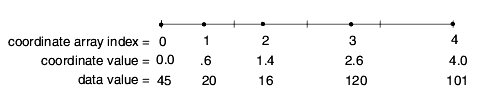
3. The number of intervals in dims_in is 4 and the number of intervals in dims_out is 3, so the ratio of the intervals between nodes dims_in: dims_out is 4 /3 or 1.333. Therefore, the four indices for dims_out are 0, 1.333, 2.666, and 3.999.
5. The result of using the coordinates and node data in the input field at these index values as the coordinates and node data for the output field is:
- The input must contain a structured mesh object (Mesh_Struct, Mesh_Rect, or Mesh_Unif), and a single Node_Data object. The mesh can be 1D, 2D, or 3D.
- A port to connect to a user interface object that contains the macro's widgets. By default, it is connected to the default user interface object in the application in which the macro is instanced. (This default connection is not drawn.)
- UItoggle. When on, the downsize factor sliders are constrained to integers rather than floats. The default is on.
- Float UIsliders to specify the scaling coefficient. The output field's values (and coordinates for irregular data) are:
- dims_out[i] = dims_in[i] / factor [i]
- where i cycles through the dims of the field, either 1D, 2D, or 3D.
- Note: factors < 1 make the output field larger. For example, a factor of .5 doubles the size of the output field.
- You control the factor for each dimension separately. The default for all factors is 8. The range for all factors is 0.0 to 12.0.
- All three controls appear no matter what the dimensionality of the input data. You only use the controls that are meaningful for the input data.
- The output field contains a new structured mesh of the same type as the input mesh, and a new Node_Data object containing the data associated with the downsized region.
- The output mesh's points array (extents) will occupy the same "space" as the input field's Mesh.
- This is a renderable version of the output field.
Libraries.Examples.Vizualization.Downsize
examples/down.v
Libraries.Examples.Visualization.Mirror_Scale
examples/mirr_scl.vinteractively draw lines on an object in a viewer
draw_line lets the user interactively draw polylines over an object in a viewer window.
- The coordinates of the picked point. This red input port should connect to a renderer's picked_obj red output port.
- A port to connect to a user interface object that contains the macro's widgets. By default, it is connected to the default user interface object in the application in which the macro is instanced. (This default connection is not drawn.)
- UItoggle. When on, the user is using the left mouse button to select a series of points on the object. Lines are drawn between each point. The default is on.
- UItoggle. When on, the user wants to select a new "first" point and begin drawing a new series of lines. When off, the user is in the middle of drawing a series of lines and any left mouse button click is a line endpoint. The default is off.
- The output is an unstructured mesh of cell type Polyline. Each cell is one line segment in the drawing.
- This is a renderable version of the output field.
perform 3D texture mapping on a 3D uniform field
excavate_brick3d is a technique for visualizing 3D uniform volume data. The volume is displayed with an X, Y, and Z slice plane. The slice removes a rectangular subvolume of the field, revealing the structures inside.
Texture mapping is much faster than the sampling techniques used by slice, particularly for large datasets. Texture mapping's point sampling is done at the resolution of the data; thus, differences in data values within a small area are not obscured as they can be with slice.
- Note: The excavate_brick3D module does not generate vertex normals by default. For more details, see Section 5.1.8, Vertex normal generation [page 5-4].
- The input is a reference to a Mesh_Unif, Dim3 field with scalar byte Node_Data.
- A colormap to provide the texture map. From Libraries.Main.Fields.Data.colormap.
- A port to connect to a user interface object that contains the macro's widgets. By default, it is connected to the default user interface object in the application in which the macro is instanced. (This default connection is not drawn.)
- UIsliders that set the X, Y, Z position of their respective slice planes. The default is the mid-point of the input field's dimensions. The range is the field's dimensions.
- UItoggles. These select whether the excavating cube should be positioned on the positive or negative axis for each of the X, Y, and Z dimensions. When on, the cube is positioned on the negative axis. The default is off.
- UItoggle. When off, only the excavating cube is drawn. When on, a texture map of the bounding faces of the volume is also drawn. The default is off.
- The output is a new Mesh and Node_Data. u, v, w textures are added.
- This is a renderable version of the output field.
excavate_brick3D creates its picture of the volume data using 3D texture mapping. In this method, the boundary of the volume has three values, u, v, w, associated with each of its vertices. Where the slice planes intersect this volume, u, v, w values are computed for the vertices of the resulting solid. These values are attached to the vertices of the output object. Viewers use the u, v, w information to create the texture-mapped rendering.
Libraries.Examples.Vizualization.Excavate_Brick: examples/excvt.v
explode individual transformations of each field in the input array of fields
explode_fields takes each input field in the input array and translates it away from the common center of all the fields, which is computed by finding the midpoint of the bounding box. You can set the amount of translation via parameters. The grid and data for the input fields are not modified, only their transformation matrices.
- Mesh[]. An array of fields to transform.
- A port to connect to a user interface object that contains the macro's widgets. By default, it is connected to the default user interface object in the application in which the macro is instanced. (This default connection is not drawn.)
- UIslider. A value specifying how much to scale the translation away from the center in the X direction. This value is in units of the bounding box of the original array of fields.
- UIslider. A value specifying how much to scale the translation away from the center in the Y direction. This value is in units of the bounding box of the original array of fields.
- UIslider. A value specifying how much to scale the translation away from the center in the Z direction. This value is in units of the bounding box of the original array of fields.
- Mesh[]. The transformed input fields.
- Renderable object corresponding to out_fld.
Libraries.Examples.Visualization.Explode_Fields
examples/explode.vcreate an array of fields from a single field based on material properties of cell sets
Each cell set in a field has an associated properties array. You may use this array to store anything related to the cell set, but it is commonly used to store material properties of the cells in the cell set.
explode_materials splits up the field into an array of fields based on the values of a particular element of the properties array. The same array index is used to look up the value in the properties array of each cell set. Each cell set with a distinct value of that property goes into a separate output field. Whether the values are equal is all that is significant, the actual values are not significant.
Note that this macro compares floating point numbers for equality; you are responsible for ensuring that the values in the material property array are bit-for-bit equal or not equal, as desired.
- Mesh. This mesh is split apart into multiple meshes on the output, according to the selected property value of each cell set.
- A port to connect to a user interface object that contains the macro's widgets. By default, it is connected to the default user interface object in the application in which the macro is instanced. (This default connection is not drawn.)
- UIslider. Selects which element of each cell set's material properties array to use to split the input. All cell sets' arrays use the same index.
- Mesh[]. An array of meshes, with other data merged from the input field.
- GroupObject. Group of renderable objects corresponding to out_fld.
Libraries.Examples.Visualization.Explode_Field
examples/explode.vextract external edges of a field to reveal inside objects
external_edges produces a wireframe representation of the outside of an unstructured mesh. You use it when you want to see objects produced by other modules that are inside an unstructured mesh (isosurfaces, streamlines, probes, and so on) while still being able to see the enclosing skeletal shape of the mesh.
- The input need only contain a mesh of any sort. Unstructured meshes pay attention to the max edge angle UIslider using DVext_edge to produce their picture. Structured meshes (Mesh_Struct, Mesh_Rect, and so on) cause DVbounds to be used, generating a simple hull of the mesh.
- A port to connect to a user interface object that contains the macro's widgets. By default, it is connected to the default user interface object in the application in which the macro is instanced. (This default connection is not drawn.)
- UIslider. A float slider that controls the accuracy of the boundary representation on the base of the angle between two adjoining faces in unstructured meshes. All edges that have an angle less than this value are represented in the output field. The range is 0.0 to 180.0. The angle used is calculated as edge_angle*3.14/180.0. The default is 5.0.
- This parameter is ignored in structured meshes.
- The output is a field containing a new unstructured Mesh of cell type Line representing the input mesh's exterior. If Node_Data was present in the input field, this output field also contains a reference to that Node_Data.
- This is a renderable version of the output field.
Libraries.Examples.Visualization.Advect
examples/advect.v
Libraries.Examples.Visualization.Cut
examples/cut.v
Libraries.Examples.Visualization.Isosurface
examples/isos.v
Libraries.Examples.Visualization.Probe
examples/probe.v
Libraries.Examples.Visualization.Stream
examples/stream.v
Libraries.Examples.Visualization.Glyph_Interp
examples/glh_intp.v
extract external faces of a field for faster rendering
external_faces produces a mesh that represents just the exterior, visible faces of an unstructured mesh. It saves memory and greatly speeds rendering because all of the unstructured mesh's many interior, hidden nodes and cells are not represented.
- Note: The external_faces module does not generate vertex normals by default. For more details, see Section 5.1.8, Vertex normal generation [page 5-4].
- The input need only contain a mesh of any sort. Unstructured meshes pay attention to the max edge angle UIslider using DVext_edge to produce their picture. Structured meshes (Mesh_Struct, Mesh_Rect, and so on) cause DVbounds to be used, generating a simple hull of the mesh.
- A port to connect to a user interface object that contains the macro's widgets. By default, it is connected to the default user interface object in the application in which the macro is instanced. (This default connection is not drawn.)
- The output is a field containing a new unstructured Mesh of cell types Quad and Tri representing the input mesh's exterior. If Node_Data was present in the input field, this output field also contains a reference to that Node_Data.
- This is a renderable version of the output field.
Libraries.Examples.Visualization.Cut
examples/cut.v
Libraries.Examples.Visualization.Isoline
examples/isol.v
Libraries.Examples.Visualization.Isovolume
examples/isov.v
Libraries.Examples.Visualization.Offset
examples/offset.vextract one cell_data component from each Cell_Data cell_set
extract_cell_component extracts one cell_data component from each Cell_Data cell_set. If there are multiple Cell_Data cell_sets, the same component is extracted from each cell_set. extrract_cell_component is the cell data equivalent of extract_component for node data.
Since the renderer draws just the first component it finds in each cell_set, you use extract_cell_component to obtain the right component from a multi-component Cell_Data field.
- The input is a field with a Mesh and Cell_Data.
- A port to connect to a user interface object that contains the macro's widgets. By default, it is connected to the default user interface object in the application in which the macro is instanced. (This default connection is not drawn.)
- UIradioBoxLabel. A series of radio buttons to pick which single component to extract. If there are multiple Cell_Data cell_sets, the same component is extracted from each cell_set. If labels are present, they are displayed.
- The output is a reference to a merged object that contains the new Cell_Data, plus references to all other unchanged objects in the input Mesh.
- This is a renderable version of the output field.
Libraries.Examples.Visualization.Cell_Data
examples/celld.vextract a single data component from a field
extract_component extracts a single data component from any Node_Data. For example, selecting the fourth component of the field (a, b, c, [e, f, g]) results in the single-component vector field ([e, f, g]).
- The input field must contain any mesh and Node_Data objects.
- A port to connect to a user interface object that contains the macro's widgets. By default, it is connected to the default user interface object in the application in which the macro is instanced. (This default connection is not drawn.)
- UIradioBoxLabel. Radio buttons to pick which data component to send to the output field. The default is the first (0th) selection. If node data labels are present, they are displayed.
- The output contains a reference to the original mesh, with new Node_Data consisting of a reference to the single extracted component in the input Node_Data. Effectively, you have "extracted" a reference to one component of the input Node_Data.
- This is a renderable version of the output field.
Libraries.Examples.Applications.IsoApp
extract selected coordinate components from mesh, after transforming
extract_coordinate_array extracts a 1D array containing the X, Y and/or Z components of the mesh's coordinates after being transformed by the mesh's transformation matrix. If X and Y are selected, it outputs X0, Y0, X1, Y1, and so on. Note that the output coordinates are not the same as the coordinates of the mesh itself; they are transformed, so they are in "world coordinates", as you would see them in the viewer.
- Mesh. The input mesh.
- A port to connect to a user interface object that contains the macro's widgets. By default, it is connected to the default user interface object in the application in which the macro is instanced. (This default connection is not drawn.)
- UIoptionBoxLabel (X, Y, Z). Selects which coordinate components to extract.
- prim[]. An array containing the extracted components.
extract selected component as an array from selected node data component
extract_data_array extracts a 1D array containing the selected component of the node data.
- Node_Data. The input Node_Data object from which to extract the component array.
- A port to connect to a user interface object that contains the macro's widgets. By default, it is connected to the default user interface object in the application in which the macro is instanced. (This default connection is not drawn.)
- UIoptionBoxLabel. Selects which data component to extract.
- prim[]. An array containing the extracted component.
- string. The label of the selected component.
create a mesh without any data
extract_mesh outputs the same mesh as the input, but with no node data (nnode_data=0).
- Mesh+Node_Data. The output mesh is copied from this input.
- Mesh. Contains only the mesh part of the input field.
- Renderable object corresponding to out_fld.
extract a scalar data element from a field's vector component
extract_scalar extracts a single scalar data element from a vector component of a field with Node_Data. For example, selecting the second vector element of the fourth component of the field (a, b, c, [e, f, g]) returns the field (f).
- The input field need only contain Node_Data. One of its components should be a vector. If a mesh is present, it is passed through unchanged as a reference in the output field.
- A port to connect to a user interface object that contains the macro's widgets. By default, it is connected to the default user interface object in the application in which the macro is instanced. (This default connection is not drawn.)
- UIradioBoxLabel. Radio buttons to pick which of the components to display in the vector component selection below. The default is the first (0th) selection. If node data labels are present, they are displayed.
- A selection to pick which vector element of a component to extract.
- The output is a field with a new Node_Data consisting of the extracted vector element. If a mesh was present in the input field, it is included in the output field as a reference to the original mesh.
- If a mesh was present, this is a renderable version of the output field. Otherwise, rendering objects generate an error.
produce a mesh with cells extruded in the Z direction based on their cell data values and optionally shrunk relative to their geometric centers
extrude_cells creates a new mesh, each cell of which is extruded in Z direction based on the selected height data (cell data) component. Optionally, cells can be shrunk relative to their geometric center (which is a point computed by averaging coordinates for all nodes in a cell). The height of extrusion is controlled by the height scale parameter. Shrink option and shrink scale is controlled by the shrink cells and shrink factor parameters. The sides of an extruded cell can optionally be created and colored based on the draw skirts and color skirts parameters.
- The input must contain any type of mesh plus Cell_Data.
- A port to connect to a user interface object that contains the macro's widgets. By default, it is connected to the default user interface object in the application in which the macro is instanced. (This default connection is not drawn.)
- UIradioBoxLabel. Radio buttons to pick which input Cell_Data component to use as a height value for each cell. The default is the first (0th) component. If cell data labels are present, they are displayed.
- UIslider. A float slider to adjust the height of extruded cells. The default is 1.0.
- UItoggle. If on, the module computes new coordinates for the extruded cell's nodes based on the shrink factor value that specifies the scale relative to the geometric centers of each cell. The default is off.
- UIslider. A float slider that adjusts the factor by which cells are scaled. The value of scale factor specifies scale relative to the geometric centers of each cell and can vary from 0 to 1, a value of 0 producing totally shrunken cells, and a value of 1 producing full size cells. The default is 0.8. The range is 0.0 to 1.0.
- UItoggle. If on, the sides (skirts) of extruded cells are created. The default is on.
- UItoggle. If on, the sides (skirts) of extruded cells are colored. The default is
off.
- The output field contains a new mesh that is created by extruding and optionally shrinking cells in the input field. It also contains a Cell_Data that was present in the input field.
- This is a renderable version of the output field.
Libraries.Examples.Visualization.Extrude_Cells
examples/extrude.vconvert an array of fields to a Multi_Block object
fields_to_mblock takes an array of fields and converts it to a Multi_Block object by adding the ancillary information kept by the Multi_Block object.
- Mesh_Struct+Node_Data+Cell_Data_Struct. The input array of fields.
- Multi_Block. The resulting multiblock dataset.
Libraries.Examples.Visualization.Multi_Block
examples/mblock.vfilter 1D data by convolving with a specified filter kernel array
filter_1D takes as its input an object that has a Node_Data subobject and performs filtering (convolution) of data values based on an array of kernels. The kernels array can be a float array of any size. The module internally normalizes the kernels array so that the sum of its elements always equals one.
filter_1d outputs the input mesh with new node data containing the convolved values.
The first output value comes from overlaying the middle element of the kernel with the first data value and performing the sum of products, and so on.
- Mesh+Node_Data. The 1D field containing the data to filter.
- float[]. Array of floats describing the filter kernel. This array is convolved with the in_field data to produce the output. Note that this array is automatically normalized so the sum of its values is 1.
- A port to connect to a user interface object that contains the macro's widgets. By default, it is connected to the default user interface object in the application in which the macro is instanced. (This default connection is not drawn.)
- UIradioBoxLabel. Selects which component of the data to filter.
- Mesh+Node_Data. Contains the filtered data.
- Renderable object corresponding to out_fld.
take an array of glyphs as input and output glyphs at nodes using node data as an index into the glyph array
geo_glyph takes an input field and an array of glyphs, and draws one glyph at each node location of the in_field. The glyph drawn is selected by using the data at that node as an index into the glyph array.
If normalize is off, floating point values are converted to integers by truncation. If normalize is on, the data range is mapped to the number of glyphs so that each glyph represents the same fraction of the data range.
If the data is out of the bounds of the glyph array, the minimum or maximum glyph is drawn, as appropriate.
The glyphs' colors are determined by the color parameters unless the glyphs themselves provide node data for coloring, and their size is scaled by the scale parameter. Their orientation is unchanged.
- Mesh+Node_Data. The field on which the glyphs are plotted.
- Mesh[]. The array glyphs to plot.
- A port to connect to a user interface object that contains the macro's widgets. By default, it is connected to the default user interface object in the application in which the macro is instanced. (This default connection is not drawn.)
- UIslider. Scales glyph size (X, Y and Z).
- UIslider. Sets color for glyphs.
- UIslider. Sets color for glyphs.
- UIslider. Sets color for glyphs.
- UItoggle. When on (1), the range of the data is matched to the number of glyphs so that each glyph represents an equal part of the range. When off (0), the data is used directly as an index into the glyph array.
- Mesh+Node_Data. Contains the output glyphs.
- Renderable object corresponding to out_fld.
Libraries.Examples.Visualization.geo_glyph
examples/g_glyph.vproduce a geometric object (glyphs) at nodal locations of an input field
glyph places a geometrical object at each node of an input field so that node locations are easily identified. The glyph can be sized and colored according to the selected data component at each node. If the glyph is an arrow in a vector field, for example, it generates a hedgehog.
- The input must contain any type of mesh plus Node_Data.
- Grid. This is simply a mesh describing the geometry of the glyph. Any mesh can be used (for example, that of a teapot) but for convenience you can use the Geometries such as Arrow1 (wireframe arrow), Arrow2 (solid arrow), or Cross3D (XYZ crosshairs) to generate the glyph.
- A port to connect to a user interface object that contains the macro's widgets. By default, it is connected to the default user interface object in the application in which the macro is instanced. (This default connection is not drawn.)
- UIradioBoxLabel. Radio buttons to pick which input Node_Data component to use to scale and distort the glyph, as controlled by Mode. The default is the
- first (0th) component. If node data labels are present, they are displayed.
- UIradioBoxLabel. Radio buttons to pick which input Node_Data component to use to color the glyph. If map component is equal to glyph component and the map component is a vector, the color represents the magnitude of the vector. If node data labels are present, they are displayed. The default is the first (0th) component.
- UIradioBoxLabel. A radio box that establishes how glyphs are rendered to represent the data values. The choices are:
Scale the glyph set by glyph component by the magnitude of the vector at that position. Also rotate the glyph in X, Y, (and Z) by the first, second, (and third) vector subcomponent values at that position. For example, a Cross3D in_probe would be rotated to reflect the vector values.
Scale the glyph set by glyph component in X, Y, (and Z) by the first, second, (and third) vector subcomponent values at that position. For example, a Cross3D in_probe's three lines would be individually scaled to match the vector values.
- UItoggle. If off, the sizes of the glyphs are proportional to the magnitude of the data component values at each node. If on, all glyphs are the same size. The default is off.
- UIslider. A float slider to adjust the sizes of the glyphs. The default is 1.0. The range is -10 to 10.
- The output field contains a new unstructured mesh (mesh type Mesh) that is the meshes of all the glyphs. It also contains a new Node_Data consisting of the magnitude of the selected component's data values if map component is a vector, or the value of the map component if the map component is a scalar.
- This is a renderable version of the output field.
Libraries.Examples.Visualization.Glyph_Interp
examples/glh_intp.v
Libraries.Examples.Visualization.Advect
examples/advect.v
Libraries.Examples.Visualization.Probe
examples/probe.vcompute the vector gradient of a vector field
gradient computes the vector gradient of a field with any mesh type.
- The input must be a field with any type of mesh and Node_Data. At least one of the Node_Data's components must be a scalar.
- A port to connect to a user interface object that contains the macro's widgets. By default, it is connected to the default user interface object in the application in which the macro is instanced. (This default connection is not drawn.)
- UIradioBoxLabel. Radio buttons to pick which component of in_field to use to compute the gradient. You must pick a scalar component. The default is the first (0th) component. If node data labels are present, they are displayed.
- The output field contains a new Node_Data that has a three-element vector float value at each node representing the gradient. Its mesh is a reference to the input mesh.
- This is a renderable version of the output field.
The algorithm used to compute the gradient in structured meshes is a finite difference approximation based on a central difference scheme. For unstructured meshes, the function is based on the cell shape functions and their derivatives.
In both cases, the equation used to compute the gradient is:

Libraries.Examples.Vizualization.Grad
examples/grad.vinterleave elements of several arrays into a 2D array
These modules interleave elements from several arrays into a 2D output array. The input arrays may have any dimensionality, but they are treated as 1D, in memory order. All input arrays should have the same total size. The output array contains one element from each array in order, followed by the next element from each array, and so on.
For example, this can be used to create an XYZ coordinate array from separate X, Y, and Z arrays.
- prim[]. One of the input arrays.
- prim[]. One of the input arrays.
- prim[]. One of the input arrays.
- prim[]. One of the input arrays.
- prim[][N]. The output array containing the interleaved data.
samples cell data of one field at the node locations of another "probe" field
interp_cell_data uses the node coordinates specified in the input mesh (in_probe) as a set of sample points for the in_field. For each sample point, it locates the cell containing that point in the in_field, and uses the (possibly vector) value of the given component in that cell as the node data in the output field.
If there is no cell in in_field containing a given sample point, a null data value is used.
- Mesh+Cell_Data. This field is sampled at the locations determined by the nodes of in_probe.
- Mesh. The node coordinates of this field define the sample points for interpolating in_field.
- A port to connect to a user interface object that contains the macro's widgets. By default, it is connected to the default user interface object in the application in which the macro is instanced. (This default connection is not drawn.)
- UIradioBoxLabel. Which data component to interpolate.
- Mesh+Node_Data. The sampled field data.
- Renderable object corresponding to out_fld.
use coordinates from a probe mesh as sample points to interpolate data in a field
interp_data uses the coordinates specified in an input mesh (in_probe) as a set of sample points for a field. It takes each set of coordinates in the mesh (the sample points), locates these same coordinates in the input field, then calculates what the interpolated data value of the selected component would be at that exact location based on the values of the same component in the adjacent nodes.
- The input is any mesh type with Node_Data.
- Any mesh whose coordinates represent the sample points.
- To create this sampling mesh you could, for example, use the plane object in Geometries.Plane, Geometries.FPlane, or the slice macro.
- A port to connect to a user interface object that contains the macro's widgets. By default, it is connected to the default user interface object in the application in which the macro is instanced. (This default connection is not drawn.)
- UIoptionBoxLabel. A set of option buttons to pick which data components of the input field to interpolate. The default is the first (0th) component. If node data labels are present, they are displayed.
- The output is a field that is a reference to the merge of the input probe's in_probe mesh, and a new Node_Data object with values consisting of the interpolated component values.
- This is a renderable version of the output field.
Structured fields use trilinear interpolation. Unstructured fields use shape function interpolation.
Libraries.Examples.Vizualization.Glyph_Interp
examples/glh_intp.v
Libraries.Examples.Applications.StreamApp
examples/stream_l.vshow an arbitrarily oriented and shaped texture mapped sample of a 3D uniform field
interp_texture3D creates a texture mapped picture of the surface of any mesh where it intersects a 3D uniform field. The sampling object can be moved through the volume in any direction. Output is generated every time the sampling object moves.
interp_texture3D differs from cut_texture3D in the following ways:
- It can texture map any object, not just a slicing plane. This sampling object can be moved in any direction with its Transformation Editor panel, not just orthogonal to the X axis.
- It only displays the texture mapped sampling object, not the exterior surfaces of the volume.
Texture mapping is much faster than the sampling techniques used by the slice modules, particularly for large datasets. The point sampling done by the texture mapping technique is always done at the resolution of the data; thus differences in data values within a small area are not obscured as they can be with slice.
- The input must be a field with a Mesh_Unif, Space3, Dim3, and Node_Data.
- The sampling object. This is generated by one of the Geometry objects such as Plane or Box. The sampling object should come with its own Transformation panel that controls object rotation, translation, and scale, as well as controls to specify its size when it is connected to the default user interface object in the application in which the macro is instanced.
- A colormap to provide the texture map. From Libraries.Main.Fields.Data.colormap.
- A port to connect to a user interface object that contains the macro's widgets. By default, it is connected to the default user interface object in the application in which the macro is instanced. (This default connection is not drawn.)
- The output field contains a new mesh object that is the texture mapped slice. It has the same type as the input mesh. It has a new Node_Data containing the texture mapping u, v, w values.
- This is a renderable version of the output field.
interp_texture3D creates its picture of the volume data using 3D texture mapping. In this method, the boundary of the volume has three values, u, v, w, associated with each of its vertices. Where the slice planes intersect this volume, u, v, w values are computed for the vertices of the resulting solid. These values are attached to the vertices of the output object. Viewers use the u, v, w information to create the texture-mapped rendering.
Libraries.Examples.Vizualization.Interp_Texture3D
examples/intrptxt.vcreate a surface of constant value at a picked probe location
iso_probe creates a surface of a given level value in a field at a probe position. This probe position is picked either interactively with the left mouse button, or specified through a Transformation Editor. This surface is, in effect, a 3D contour.
This isosurface of one component is colored by the value of another component, for example, the isosurface of density colored by temperature. The selected iso_probe component must be scalar. You use iso_probe when you want to see a graphic depiction of the locations of a particular data value at a particular location in a 3D field.
- The input is any mesh with Node_Data. The mesh can be of any defined type (Mesh, Mesh_Struct, Mesh_Unif, Mesh_Rect). At least one of the components must be scalar.
- Grid. A glyph to represent the probe object. This is simply a mesh describing the geometry of the glyph. Any mesh can be used, for example, that of a teapot, but for convenience you can use the predefined glyphs in Geometries (for example, Cross3D or Arrow1) to generate the mesh.
- This input connects to a renderer's picked_obj red output port. It informs iso_probe which object has been picked to probe.
- A port to connect to a user interface object that contains the macro's widgets. By default, it is connected to the default user interface object in the application in which the macro is instanced. (This default connection is not drawn.)
- UIradioBoxLabel to pick which component to isosurface. The selected component must be scalar or the message "iso: first component is not scalar" is written to stderr. The default is the first (0th) component. If node data labels are present, they are displayed.
- UIradioBoxLabel to pick a component that will map onto the isosurface, for example, map pressure value onto a density isosurface. The selection does not have to be scalar. The default is the first (0th component). If node data labels are present, they are displayed. Where the isosurface does not exactly intersect a node, the data value is linearly interpolated based on the surface's distance from the adjacent nodes.
- UItoggle. If off, the size of the probe is proportional to the data component values at each node. If on, the probe is the probe scale size. The default is off.
- UIslider. A float slider to adjust the size of the probe. The default is 1.0. The range is -10.00 to 10.
- UIslider. A float slider. This is an output parameter only-it displays the value of the data at the probe's location. Where the probe does not fall exactly on a node, the value is interpolated from the values of adjacent nodes.
Note that the value displayed is accurate if the selected component was a scalar. If it was a vector, you see only the value of that component's first vector element.
- XformEditor. A transformation editor used to place the probe within the input field if you do not want to use the left mouse button to point and click a position.
- The output field is an unstructured Mesh of cell type Tri that represents the 3D contour surface. Its Node_Data is the interpolated values of the map_component component along the isosurface.
- This output is of marginal utility. It contains the mesh of the probe object and Node_Data that is the value of the data at the probe's current location.
- This is a renderable version of the output field.
- This is a renderable version of the probe object.
iso_probe uses the Marching Cubes algorithm to construct the isosurface. See W. Lorensen and H. Cline, "Marching Cubes: A High Resolution Surface Reconstruction Algorithm." Computer Graphics 21(4) (SIGGRAPH Proceedings, 1987), July, 1987, pp. 163-169.
This algorithm has a known limitation; where there are two possible paths that the isosurface could take through a cell, only one is the correct path. If isosurface picks the wrong path, a discontinuity appears as a hole in the surface.
Libraries.Examples.Vizualization.Iso_Probe: examples/isop.v
create contour lines of constant value
isoline creates contour lines of a given level value or values in a field. The contour lines are colored by the level value. The selected component must be scalar. You use isoline when you want to see a graphic depiction of the locations of a particular data value in a field.
- The input is any mesh with Node_Data. The mesh must be a surface (nspace = 2). The surface can exist in 2D or 3D. No checking is done to ensure that the mesh is 2D. 3D meshes do not generate output. At least one of the components must be scalar.
- A port to connect to a user interface object that contains the macro's widgets. By default, it is connected to the default user interface object in the application in which the macro is instanced. (This default connection is not drawn.)
- UIradioBoxLabel. A set of radio buttons to pick which component to compute the isolines for. The selected component must be scalar or the message "isoline: first component is not scalar" is written to stderr. The default is the first (0th) component. If node data labels are present, they are displayed in the UIradioBox.
- UIslider. Number of isolines to produce. The lines are evenly spaced between the min and max levels. Default number is 10.
- UIslider. Float slider to set the minimum isoline level. The default is the selected component's min * 0.7 + max * 0.3. The range is from min to max. The data type of the slider is converted to the data type of the node data before use.
- UIslider. Float slider to set the maximum isoline level. The default is the selected component's min * 0.3 + max * 0.7. The range is from min to max. The data type of the slider is converted to the data type of the node data before use.
- UItoggle. When on, the isolines are colored by the data value. The default is on.
- The output field is a new unstructured Mesh of cell type Line that represents the contour lines. It has a new Node_Data whose value at each line is the level value of that line.
- This is a renderable version of the output field.
For each "cell" of the field, a straight line is created connecting locations on the cell's edges with an interpolated value equal to the iso level. The interpolation is linear.
Libraries.Examples.Visualization.Isoline
examples/isol.vcreate a local line of constant value at a picked probe location
isoline_trace is similar to isoline. It creates a line of a given level value in a 2-space field at a probe position. This probe position is picked interactively with the left mouse button or specified through a Transformation Editor. This line is, in effect, a 2D contour.
isoline_trace differs from isoline in that it does not isoline the entire volume of the field. Rather, beginning from the picked position, it builds an isoline by checking the values of adjacent cells until either no more adjacent cells have the same value, it hits the limits of the field, or the line is closed. Thus, isoline_trace creates local isolines.
The isoline is colored by the value of the selected iso component. That component is also written to the output Node_Data.
- The input is any Mesh_Struct (Mesh_Struct, Mesh_Rect, or Mesh_Unif) with Node_Data. The mesh must be a surface (nspace = 2). The surface can exist in 2D or 3D. No checking is done to ensure that the mesh is 2D. 3D meshes do not generate output. At least one of the components must be scalar.
- Grid. This input is a Grid representing any kind of probe object. Such objects are found in Geometries, such as Arrow, or Cross3D. In turn, the probe macro icon's red input port must connect to the renderer's picked_obj red output port.
- A port to connect to a user interface object that contains the macro's widgets. By default, it is connected to the default user interface object in the application in which the macro is instanced. (This default connection is not drawn.)
- UIradioBoxLabel to pick which component to isosurface. The selected component must be scalar or the message "iso: first component is not scalar" is written to stderr. The default is the first (0th) component. If node data labels are present, they are displayed.
- UIslider. This widget is output only. A float slider that reports the value for which the isoline is being drawn.
- The output field is an unstructured Mesh of cell type Line that represents the 2D contour lines. Its Node_Data is the interpolated values of the iso component along the isolines.
- This is a renderable version of the output field.
isoline_trace uses the Marching Cubes algorithm to construct the isosurface. See W. Lorensen and H. Cline, "Marching Cubes: A High Resolution Surface Reconstruction Algorithm." Computer Graphics 21(4) (SIGGRAPH Proceedings, 1987), July, 1987, pp. 163-169.
This algorithm has a known limitation. There are cases where there are two possible paths that the isosurface could take through a cell, and only one is the correct path. If isosurface picks the wrong path, a discontinuity appears as a hole in the surface.
create a surface of constant value
isosurface creates a surface of a given constant value level in a field. This surface is, in effect, a 3D contour. This isosurface of one node data component can be colored by the value of another node data or cell data component (for example, the isosurface of density colored by temperature). The selected iso component must be scalar. You use isosurface when you want to see a graphic depiction of the locations of a particular data value in a 3D field.
- The input is any mesh with Node_Data. The mesh can be of any defined type (Mesh, Mesh_Struct, Mesh_Unif, Mesh_Rect). At least one node data component must be scalar.
- A port to connect to a user interface object that contains the macro's widgets. By default, it is connected to the default user interface object in the application in which the macro is instanced. (This default connection is not drawn.)
- UIradioBoxLabel. Radio buttons to pick which component to isosurface. The selected component must be scalar or the message "iso: first component is not scalar" is written to stderr. The default is the first (0th) component. If node data labels are present, they are displayed.
- UIoptionBoxLabels. Option buttons to pick which components of node data to map onto output surface (for example, map pressure value onto a density isosurface). Multiple components or none can be slected. The selected component(s) can be scalars or vectors. The default is the first (0th) component. If node data labels are present, they are displayed. The data values are linearly interpolated based on the surface's distance from the adjacent nodes.
- UIoptionBoxLabels. Option buttons to pick which components of cell data to map onto output surface (for example, map pressure value onto a density isosurface). Multiple components or none can be slected. The selected component(s) can be scalars or vectors. e a scalar. The default is the first (0th) component. If cell data labels are present, they are displayed. The data values for each triangle of the output mesh are copied from original cells.
- UIslider. Float slider to set the isosurface level. The default is the selected component's (min+max)/2. The range is from min to max. The data type of the slider is converted to the data type of the node data before use.
- The output field is an unstructured triangular mesh of that represents the contour surface. It may optionaly have node and/or cell data.
- This is a renderable version of the output field.
isosurface uses the Marching Cubes algorithm to construct the isosurface. See W. Lorensen and H. Cline, "Marching Cubes: A High Resolution Surface Reconstruction Algorithm." Computer Graphics 21(4) (SIGGRAPH Proceedings, 1987), July, 1987, pp. 163-169.
This algorithm has a known limitation. There are cases where there are two possible paths that the isosurface could take through a cell, and only one is the correct path. If isosurface picks the wrong path, a discontinuity appears as a hole in the surface.
Libraries.Examples.Visualization.Isosurface
examples/isos.v
Libraries.Examples.Visualization.Crop
examples/crop.v
Libraries.Examples.Visualization.Downsize
examples/down.v
Libraries.Examples.Visualization.Probe
examples/probe.v
Libraries.Examples.Applications.IsoApp
examples/iso.vcreate a local surface of constant value at a picked probe location
isosurface_trace is similar to isosurface. It creates a surface of a given level value in a field at a probe position. This probe position is picked interactively with the left mouse button or specified through a Transformation Editor. This surface is, in effect, a 3D contour.
isosurface_trace differs from isosurface in that it does not isosurface the entire volume of the field. Rather, beginning from the picked position, it builds an isosurface by checking the values of adjacent cells until either no more adjacent cells have the same value, it hits the limits of the field, or the surface is closed. Thus, isosurface_trace creates local isosurfaces.
The isosurface of one component is colored by the value of the selected map component (for example, the isosurface of density colored by temperature). That map component is also written to the output Node_Data.
- The input is any Mesh_Struct (Mesh_Struct, Mesh_Rect, or Mesh_Unif) with Node_Data. At least one of the components must be scalar.
- Grid. This input is a Grid representing any kind of probe object. Such objects are found in Geometries, such as Arrow, or Cross3D. In turn, the probe macro icon's red input port must connect to the renderer's picked_obj red output port.
- A port to connect to a user interface object that contains the macro's widgets. By default, it is connected to the default user interface object in the application in which the macro is instanced. (This default connection is not drawn.)
- UIradioBoxLabel to pick which component to isosurface. The selected component must be scalar or the message "iso: first component is not scalar" is written to stderr. The default is the first (0th) component. If node data labels are present, they are displayed.
- UIradioBoxLabel to pick a component that will map onto the isosurface (for example, map pressure value onto a density isosurface). The selection does not have to be scalar. The default is the first (0th component). If node data labels are present, they are displayed. Where the isosurface does not exactly intersect a node, the data value is linearly interpolated based on the surface's distance from the adjacent nodes.
- UIslider. This widget is an output display only. It ignores input. A float slider that reports the value found at the picked location for which an isosurface has been drawn.
- The output field is an unstructured Mesh of cell type Tri that represents the 3D contour surface. Its Node_Data is the interpolated values of the map component along the isosurface.
- This is a renderable version of the output field.
isosurface_trace uses the Marching Cubes algorithm to construct the isosurface. See W. Lorensen and H. Cline, "Marching Cubes: A High Resolution Surface Reconstruction Algorithm." Computer Graphics 21(4) (SIGGRAPH Proceedings, 1987), July, 1987, pp. 163-169.
This algorithm has a known limitation. There are cases where there are two possible paths that the isosurface could take through a cell, and only one is the correct path. If isosurface picks the wrong path, a discontinuity appears as a hole in the surface.
Libraries.Examples.Vizualization.Iso_Trace
examples/isotrc.vcreate a volume of the data inside or outside an isosurface
isovolume cuts the input mesh using an isosurface of the selected component with a specified iso level value. It outputs the portion of the mesh that is on one side of the cutting isosurface, along with the data for one or more components. The dimensionality of the resulting mesh (1D, 2D or 2D) is the same as dimensionality of original mesh. For example, if you had an MRI scan of a cranium, represented as 3D volume field, you could set iso level to the value for bone, toggle Above, and produce a 3D field that was all the tissue inside the skull.
- Note: The isovolume module does not generate vertex normals by default. For more details, see Section 5.1.8, Vertex normal generation [page 5-4].
- The input is any mesh with Node_Data. At least one of the components must be scalar.
- A port to connect to a user interface object that contains the macro's widgets. By default, it is connected to the default user interface object in the application in which the macro is instanced. (This default connection is not drawn.)
- UIradioBoxLabel. Radio buttons to pick which component to use to construct the isosurface. The selected component must be scalar or the message "iso: first component is not scalar" is written to stderr. The default is the first (0th) component. If node data labels are present, they are displayed.
- UIoptionBoxLabels. Option buttons to pick which components of node data to map onto output surface or volume (for example, map pressure value onto a density isovolume). Multiple components or none can be slected. The selected component(s) can be scalars or vectors. The default is the first (0th) component. If node data labels are present, they are displayed. The data values are linearly interpolated based on the surface's distance from the adjacent nodes.
- UIoptionBoxLabels. Option buttons to pick which components of cell data to map onto output surface or volume (for example, map pressure value onto a density isosurface). Multiple components or none can be slected. The selected component(s) can be scalars or vectors. e a scalar. The default is the first (0th) component. If cell data labels are present, they are displayed. The data values for each cell of the output mesh are copied from original cells.
- UItoggle that selects whether the extracted volume is inside or outside the isosurface. Above turned on means that output values are greater than the cut level. The default is on.
- UIslider. Float slider to set the isosurface level. The default is the selected component's (min+max)/2. The range is from min to max. The data type of the slider is converted to the data type of the node data before use.
- The output field is a new mesh of the same dimensionality as the input that represents the new volume. Its new node and/or cell sata are the values of the selected map components. It does contain a reference to the input field's xform.
- This is a renderable version of the output field.
isovolume uses the "Marching Cubes" algorithm to construct the isosurface. See W. Lorensen and H. Cline, "Marching Cubes: A High Resolution Surface Reconstruction Algorithm." Computer Graphics 21(4) (SIGGRAPH Proceedings, 1987), July, 1987, pp. 163-169.
Libraries.Examples.Visualization.Isovolume: examples/isov.v
Libraries.Examples.Visualization.IsoVolume_2D: examples/isov2uni.v
Libraries.Examples.Visualization.Volume_Integral: examples/vintgr.vfit a polynomial of specified order using the least squares method
least_squares fits a polynomial of a given order to an input data set. The input consist of (x, y) pairs, where the X's are the 1D mesh coordinates of the nodes, and the Y's are the node_data values. These points are fit to a polynomial of the desired degree. Two outputs are produced; out_coeff is an array containing the n+1 coefficients of the resulting polynomial, and out_fld is the fit Y values computed by evaluating the polynomial at each X point.
- Grid+Node_Data+Scalar. 1D field containing data to fit.
- A port to connect to a user interface object that contains the module's widgets. By default, it is connected to the default user interface object in the application in which the macro is instanced. (This default connection is not drawn.)
- UIradioBoxLabel. Which component of the data to fit to the polynomial.
- UIslider. Order of the polynomial to fit to the data-1=linear, 2=quadratic, and so on.
- double[order+1]. The coefficients of the resulting polynomial, in order from least significant (constant term) to most significant (highest power).
- Mesh+Node_Data. Node_Data values are the polynomial evaluated at the points on the mesh.
- Renderable object corresponding to out_fld.
periodically increment an output value
Loop initializes its count output to its start value, and periodically increments it by incr. When the value reaches or exceeds the end value, the done flag is set unless cycle is nonzero, in which case the loop count is reset to the start value and another loop starts. If the increment is negative, the end test becomes whether the current count is less than or equal to the end value, so loops can go in either direction.
The value is updated whenever all other modules are done executing and the network reaches a quiescent state.
If cycle is 0, the final value is always exactly the end value, even if the increment plus the next-to-last value would have gone past the end value.
The loop can be interrupted at any time by setting run to 0.
- A port to connect to a user interface object that contains the macro's widgets. By default, it is connected to the default user interface object in the application in which the macro is instanced. (This default connection is not drawn.)
- UItoggle. When nonzero, the loop runs, incrementing as usual. When the loop reaches the end, the run parameter is automatically set to zero unless the cycle parameter is nonzero. If run is set to zero while the loop is running, it stops at the current value until run is set to one.
- UItoggle. When set to nonzero, the start value is loaded into the current count, but the loop does not stop running. It is automatically reset to 0after the reset is done.
- UItoggle. When nonzero, the count is reset to the start when it reaches the end, and the loop continues endlessly as long as run is nonzero. When cycle is zero, the count stops at the end value.
- UIfieldTypein. The starting value for the loop. Reset causes this value to be stored into the loop count, and if cycle is nonzero it is reloaded each time the current value passes the end value.
- UIfieldTypein. The ending value for the loop.
- UIfieldTypein. The increment added to the value each time through the loop.
- UIfieldTypein. The current value for the loop.
- Note that this value does not count the number of loops executed, unless start is 0.0 and incr is 1.0; it accumulates the current value of the loop.
- Automatically set to 1 when the loop finishes. Never set to 1 if cycle is true.
calculate the magnitude of a vector field
magnitude calculates the magnitude of a vector field.
- The input is any mesh with Node_Data.
- A port to connect to a user interface object that contains the macro's widgets. By default, it is connected to the default user interface object in the application in which the macro is instanced. (This default connection is not drawn.)
- UIradioBoxLabel. Radio buttons to pick which component to use to calculate the magnitude. This component can contain one-, two-, or three-vector subcomponents. The default is the first (0th) component. If node data labels are present, they are displayed.
- The output field is a reference to a new object that is the merge of the new Node_Data, plus a reference to the original input mesh. This new Node_Data is a scalar representing the magnitude.
- This is a renderable version of the output field.
The equation used to compute the magnitude is:
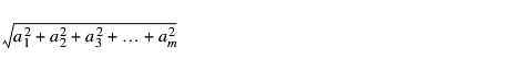
where a1, a2, and so on are the individual vector subcomponents within the selected component.
convert a Multi_Block object to an array of fields
mblock_to_fields extracts the array of fields contained in the Multi_Block object.
- Multi_Block. The input multiblock dataset.
- Mesh_Struct+Node_Data+Cell_Data_Struct. The array of fields extracted from multi_block.
create the mirror image of an unstructured Mesh
mirror generates a mesh that is the mirror image of the input mesh by reflecting the mesh about the X, Y, and/or Z plane. You can control each independently. Mirroring is useful for visualizing axisymmetric problems.
- The input is any mesh. Any Node_Data that is present is ignored.
- A port to connect to a user interface object that contains the macro's widgets. By default, it is connected to the default user interface object in the application in which the macro is instanced. (This default connection is not drawn.)
- UItoggles. When on, its respective axis is mirrored. The default for all is on.
- The output field is a reference to the input field, but with a new, modified xform transformation matrix object.
- This is a renderable version of the output field.
Libraries.Examples.Visualization.Mirror_Scale
examples/mirr_scl.vData mappers that create Node_Data objects given data array(s)
The node_scalar and node_vector macros create Node_Data objects that can merge with a Mesh object to create a field. A Node_Data object represents the values of some dataset at the node points of a field, while the Mesh represents the locations of that field's nodes in space.
These macros simplify the process of generating field data by reducing the amount of data you must supply to create a field. Usually the output of one of these macros is combined, using combine_mesh_data, with the output of one of the mesh mapper macros to create a field.
- array of any primitive type. Contains the node data to use. For node_scalar, the array's length should be the number of nodes in the dataset. For node_vector, the array's length should be nnodes * veclen.
- Node_Data. The node data object containing the given data array.
Section 5.72, radius_data, rgb_data, argb_data, node_colors, node_normals, node_uv, node_uvw, pick_data [page 5-171]
deform a mesh by data vector at each node
offset "physically" deforms a mesh by the values of a one-, two-, or three-vector component located at each node. The first element of the vector translate's the node's X coordinate, the second (if present) translates the Y coordinate, and the third (if present) translates the Z coordinate. The magnitude of each translation is proportional to the values at the nodes multiplied by a scaling factor.
- The input is any mesh with Node_Data. Its components can be a one-, two-, or three-element vector.
- A port to connect to a user interface object that contains the macro's widgets. By default, it is connected to the default user interface object in the application in which the macro is instanced. (This default connection is not drawn.)
- UIradioBoxLabel. Radio buttons to pick which component to use as the three-element vector that defines the offset. The default is the first (0th) component. If node data labels are present, they are displayed.
- UIslider. A float slider used to scale the degree of distortion caused by the vector component. The default is 1.0. The range is -10.0 to 10.0.
- The output is a new field containing as its mesh the original mesh distorted by the vector component times the scaling factor, and containing as its Node_Data a reference to the input Node_Data. A generic input Mesh creates a Mesh output. Mesh_Struct, Mesh_Unif, or Mesh_Rect input creates Mesh_Struct output.
- This is a renderable version of the output field.
Libraries.Examples.Visualization.Offset
examples/offset.v
Libraries.Examples.Visualization.Surf_plot
examples/surf_plt.vproduce a slice of a structured field perpendicular to a coordinate axis
orthoslice subsets a structured field by extracting one slice plane. The slice plane can only be orthogonal to the X, Y, or Z axis.
- The input must contain a structured mesh (mesh type Mesh_Struct, Mesh_Unif, or Mesh_Rect) and Node_Data. The input can be 1D, 2D, or 3D.
- A port to connect to a user interface object that contains the macro's widgets. By default, it is connected to the default user interface object in the application in which the macro is instanced. (This default connection is not drawn.)
- UIslider. An integer slider. Selects which axis (X = 0, Y = 1, Z = 2) the orthoslice is perpendicular to. The default is 0. If the field is 1D or 2D, three values are still displayed. Select the values meaningful for the input data.
- UIslider. An integer slider. Selects which plane to extract from the input. The default is dims[axis]/2. The range is 0 to max_dim.
- The output is a field with a new structured mesh of the same type as the input field. The mesh is the mesh of the slice. It contains the slice's Node_Data.
- This is a renderable version of the output field.
Libraries.Examples.Visualization.Orthoslice
examples/orth.v
Libraries.Examples.Visualization.Null_Data
examples/nulldt.vsubset a volume using any number of 2D uniform grids as slicing planes
plane_crop subsets a field by outputting all whole cells that are inside or outside a volume created by an unlimited number of slice planes.
- The input is a field with any Mesh. Node_Data is optional.
- An array of Plane_Grids that will slice the volume. A Plane_Grid is defined as Grid_Unif+Space2+Dim2. It is, therefore, any 2D uniform grid.
- A port to connect to a user interface object that contains the macro's widgets. By default, it is connected to the default user interface object in the application in which the macro is instanced. (This default connection is not drawn.)
- UItoggle. When on, the entire cell intersected by a plane is output. If it is off, the entire cell is not output.
- UItoggle. When on, the cells inside the slicing planes are output. If it is off, the cells outside the slicing planes are output.
- The output is a new Mesh and Node_Data that is the plane-cropped input Mesh, plus any Node_Data for the output nodes. The mesh contains a reference to the input field's xform.
- This is a renderable version of the output field.
reads a multiblock Plot3D format data file
Plot3d_Multi_Block reads a pair of files that describe a Plot3D dataset. It reads that data into an array of fields; each field describes one block of the dataset. The result can be operated on by any of the *_ARR array-of-fields macros.
The Multi_Block object contains the array of fields plus some additional information, including the number of blocks and the bounds of the dataset.
- A port to connect to a user interface object that contains the macro's widgets. By default, it is connected to the default user interface object in the application in which the macro is instanced. (This default connection is not drawn.)
- UIfileSB. Name of Plot3d xyz file.
- UIfileSB. Name of Plot3d q file.
- Multi_Block object.
- Array of fields.
Libraries.Examples.Visualization.Multi_Block: examples/mblock.v
mesh mappers that create meshes containing Point, Line or Polyline cells from coordinate and connectivity arrays
Each of these macros creates a mesh containing cells (geometric objects), given arrays containing the locations of the nodes in space and their connectivity. These macros simplify the process of generating field data by reducing the amount of data you must supply to create a field. Usually the output of one of these macros is combined, using combine_mesh_data, with the output of one of the data mapper macros to create a field.
point_mesh creates a mesh containing a cell set of type Point.
line_mesh creates a mesh containing a cell set of type Line.
line_disjoint_mesh creates disjoint lines in a cell set of type Line. It accepts two arrays, one with the start coordinates and one with the end coordinates for each line.
polyline_mesh creates a mesh containing a cell set of type Polyline. This cell set can contain multiple disconnected polylines.
- float[nnodes][nspace]. This array specifies the coordinates of the vertices of the cells. Their connectivity (for example, into lines or polylines) is specified in the connect array. For example, coord[4][2]={{0,0}, {1,0}, {1,1}, {0,1}} creates four vertices at the corners of the unit square in 2-space. In 3-space, you can add a Z coordinate value to each of the subarrays.
- int[nnodes * cell_nnodes]. For each cell, this array specifies which node in the coord array describes each vertex of that cell. The layout is by cells, with the nodes of each cell specified in the canonical cell order (see Section 2.9, Cell_Set [page 2-42] for the cell orderings for all supported cell types).
- For example, to specify the letter Z as three lines using the line_mesh macro using the example coords above, you can specify connect[6]={0,1,1,3,3,2}. The first line uses vertices 0 and 1, the second 1 and 3, and the third 3 and 2.
- The polyline_mesh macro treats the connect array differently, since it generates multiple polylines. Elements of the connect array are taken in pairs; the first and second elements are start and end indices into the coordinates array, producing a set of coordinates for each polyline strip. Polylines are drawn as connected line segments from the first coordinate to the last coordinate. So, to draw a backward C-shaped polyline using the example coords, above, you can specify connect[2]={0,3}. This uses all four coordinates in a single polyline.
- line_disjoint_mesh differs from the other *_mesh macros because it uses two coord arrays-coord1 and coord2, instead of coord and connect. Line segments are created between corresponding elements of the two arrays, which must have the same length.
- Mesh. Contains the mesh described by the input arrays.
- Renderable object corresponding to out.
Section 5.72, radius_data, rgb_data, argb_data, node_colors, node_normals, node_uv, node_uvw, pick_data [page 5-171]
Section 5.111, uniform_scalar_field, uniform_vector_field, image_field, image_field_rgb, image_field_argb, volume_field, rect_scalar_field, rect_vector_field, struct_scalar_field, struct_vector_field [page 5-278]
mesh mappers that create meshes containing Tri, Quad or Polytri cells from coordinate and connectivity arrays
Each of these macros creates a mesh containing cells (geometric objects), given arrays containing the locations of the nodes in space and their connectivity. These macros simplify the process of generating field data by reducing the amount of data you must supply to create a field. Usually the output of one of these macros is combined, using combine_mesh_data, with the output of one of the data mapper macros to create a field.
polytri_mesh creates a mesh containing a cell set of type Polytri. This may contain multiple polytriangle strips.
tri_mesh creates a mesh containing a cell set of type Tri.
quad_mesh creates a mesh containing a cell set of type Quad.
- float[nnodes][nspace]. This array specifies the coordinates of the vertices of the cells. Their connectivity (for example, into quads or triangles) is specified in the connect array. For example, coord[4][2]={{0,0}, {1,0}, {1,1}, {0,1}} creates four vertices at the corners of the unit square in 2-space. In 3-space, you can add a Z coordinate value to each of the subarrays.
- int[nnodes * cell_nnodes]. For each cell, this array specifies which node in the coord array describes each vertex of that cell. The layout is by cells, with the nodes of each cell specified in the canonical cell order (see Section 2.9, Cell_Set [page 2-42] for the cell orderings for all supported cell types).
- For example, to specify a square using the example coordinates above, provide the quad_mesh macro with connect[4]={0,1,2,3}. To specify two triangles using the example coordinates above, provide the tri_mesh macro with connect[6]={0,3,2,0,2,1}. Note that in this last case there are two triangles of three vertices each, giving six entries in the array. The triangles are specified in a counterclockwise order, as required for the canonical triangle vertex ordering.
- The polytri_mesh macro treats the connect array differently. Elements of the connect array are taken in pairs; each pair representing the start and end indices into the coordinates array for one polytriangle. If a coord array of dimensions [12][2] were provided, a connect array of the form connect[4] = {0,4,5,11} would produce two polytriangle strips: the first would contain triangles with coordinate indices {{0,1,2},{1,2,3},{2,3,4}} and the second would contain triangles with coordinate indices {{5,6,7},{6,7,8},{7,8,9},{8,9,10},{9,10,11}}.
- Mesh. Contains the mesh described by the input arrays.
- Renderable object corresponding to out.
Section 5.72, radius_data, rgb_data, argb_data, node_colors, node_normals, node_uv, node_uvw, pick_data [page 5-171]
Section 5.111, uniform_scalar_field, uniform_vector_field, image_field, image_field_rgb, image_field_argb, volume_field, rect_scalar_field, rect_vector_field, struct_scalar_field, struct_vector_field [page 5-278]
mesh mappers that create meshes containing Tet, Hex, Pyr, Prism and Polyhedron cells from coordinate and connectivity arrays
Each of these macros creates a mesh containing cells (geometric objects), given arrays containing the locations of the nodes in space and their connectivity. These macros simplify the process of generating field data by reducing the amount of data you must supply to create a field. Usually the output of one of these macros is combined, using combine_mesh_data, with the output of one of the data mapper macros to create a field.
tet_mesh creates a mesh containing a cell set of type Tet (tetrahedra).
hex_mesh creates a mesh containing a cell set of type Hex (hexahedra).
pyramid_mesh creates a mesh containing a cell set of type Pyr (pyramid).
prism_mesh creates a mesh containing a cell set of type Prism (that is, a polyhedron with two three-sided faces and three four-sided faces).
polyhedron_mesh creates a mesh containing a cell set of type Polyhedron (see the description of the poly_nodes input port.)
- float[nnodes][nspace]. This array specifies the coordinates of the vertices of the cells. Their connectivity (for example, into tetrahedra or pyramids) is specified in the connect array. For example, coord[8][3]={{0,0,0},{1,0,0},{1,1,0},{0,1,0},{0,0,1},{1,0,1},{1,1,1},{0,1,1}} creates eight vertices at the corners of the unit cube in 3-space.
- int[nnodes * cell_nnodes]. For each cell, this array specifies which node in the coord array describes each vertex of that cell. The layout is by cells, with the nodes of each cell specified in the canonical cell order (see Section 2.9, Cell_Set [page 2-42] for the cell orderings for all supported cell types).
- For example, to specify a single cube cell using the example coordinates above, provide the hex_mesh macro with connect[8] = {7,4,5,6,3,0,1,2}. Note that in this case there is one hexahedron of eight vertices. The hexahedron vertices are specified in a the order specified for the canonical hexahedron vertex ordering (See Section 2.21, Hex, Hex2 [page 2-72]).
- int[npolys]. The polyhedron_mesh macro, which actually generates polygons, needs one additional parameter-the number of nodes of each polygon. Each element of this array describes the number of nodes in the corresponding polygon in the connect array. Thus, the first poly_nodes[0] elements of the connect array describe the nodes of the first polygon, the next poly_nodes[1] elements describe the next polygon, and so on. For polyhedron_mesh, the size of the connect array should equal sum(poly_nodes).
- Mesh. Contains the mesh described by the input arrays.
- Renderable object corresponding to out.
Section 5.72, radius_data, rgb_data, argb_data, node_colors, node_normals, node_uv, node_uvw, pick_data [page 5-171]
Section 5.111, uniform_scalar_field, uniform_vector_field, image_field, image_field_rgb, image_field_argb, volume_field, rect_scalar_field, rect_vector_field, struct_scalar_field, struct_vector_field [page 5-278]
interactively show numeric data values of field at probe location
probe displays the data values present at the probe object's location in a mesh. When the probe object is not exactly on a node, the value shown is the result of an interpolation of the adjacent node data values.
- This input is a field with any mesh type and Node_Data.
- A glyph to represent the probe object. This is a mesh describing the geometry of the glyph. Any mesh can be used (that is, that of a teapot), but for convenience you can use the meshes defined in Geometries such as Arrow1, Cross2D, or Cross3D.
- This input is connected to the renderer module's picked_obj red output port. It informs probe which object has been picked to probe.
- A port to connect to a user interface object that contains the macro's widgets. By default, it is connected to the default user interface object in the application in which the macro is instanced. (This default connection is not drawn.)
- UIradioBoxLabel. Radio buttons to pick which of the input field's components to probe. The component can be scalar or vector. The default is the first (0th) component. If node data labels are present, they are displayed.
- UItoggle. If off, the size of the probe is proportional to the data component values at each node. If on, the probe is the probe scale size. The default is off.
- UIslider. A float slider to adjust the size of the probe. The default is 1.0. The range is -10.00 to 10.
- UIfieldTypein. A float. This is an output parameter only-it displays the value of the data at the probe's location. Where the probe does not fall exactly on a node, the value is interpolated from the values of adjacent nodes.
- Note that the value displayed is accurate if the selected component was a scalar. If it was a vector, you see only the value of that component's first vector element.
- A transformation editor (XformEditor). Used to place the probe within the input field.
- This output is of marginal utility. It contains the mesh of the probe object and Node_Data that is the value of the data at the probe's current location.
- This is a renderable version of the output field.
The algorithms used to interpolate the value at the probe location are trilinear interpolation for structured fields and shape functions for unstructured fields.
Libraries.Examples.Visualization.Probe: examples/probe.v
interactively probe cell data values
probe_cell interactively probes the value of a cell-based dataset, using a user-specified probe glyph. You click in the viewer (using the pick button) to select an object and a point on or in that object; that point is used to sample the object's cell data by finding which cell encloses that point, and using that cell's data value. The sampled value is shown in four ways:
- It is reported numerically in the value window.
- It is applied as node data to the glyph, which usually colors the glyph.
- It can optionally scale the glyph in X, Y and Z (if Probe Normalize is off).
- The glyph's origin is transformed to lie at the sample point.
Note that a pick object is necessary to run the module, so you must click in the viewer to set the location of the probe glyph. After the selected object is determined, you can transform the probe glyph in three ways:
- Numerically, using probe_cell's glyph transform editor.
- Interactively, by clicking on a different part of the dataset.
- Interactively, by directly manipulating the probe glyph.
- Mesh+Cell_Data. The field to probe.
- Mesh. The glyph to use to show the location of the probe point. This can be any mesh (for example, a teapot), but the simple meshes defined in Geometries such as Arrow1, Cross2D, or Cross3D are commonly used.
- GDobject_templ. A pick object which is output from a viewer.
- A port to connect to a user interface object that contains the macro's widgets. By default, it is connected to the default user interface object in the application in which the macro is instanced. (This default connection is not drawn.)
- UIradioBoxLabel. Which component of the data to probe. If the selected component is a vector, only the first element of the vector is shown.
- UItoggle. When this is on, the size of the glyph is not scaled by the probed data value. When off, the size is scaled.
- UIslider. Scales the size of the glyph in X, Y and Z. If normalize is off, both the data scale and this scale are applied.
- UIfieldTypein. The value of the cell data component at the probe point.
- The output field consists of the input glyph mesh transformed to the probe location, scaled by the scale value and optionally the data value, and with Node_Data containing the probed data value.
- Renderable object corresponding to out_fld.
data mappers that create Node_Data objects representing particular types of data
These macros output a Node_Data object with preset identifiers that tell the renderer that the data is to be used for a particular purpose. They create Node_Data objects that can merge with a Mesh object (and possibly other node data) to create a field. A Node_Data object represents the values of some dataset at the node points of a field, while the Mesh represents the locations of that field's nodes in space.
These macros simplify the process of generating field data by reducing the amount of data you must supply to create a field. Usually the output of one of these macros is combined, using combine_mesh_data and possibly combine_node_datas, with the output of one of the mesh mapper macros to create a field. These macros are subclassed from node_scalar and node_vector; the only difference is that the id member of the Node_Data object is preset to particular values.
The amount of data provided in the in_data array must match the number of nodes in the eventual field to be constructed.
- Specifies scalar data (one value per node). Whenever the nodes in the resulting field are rendered as spheres, this data will control the radius of the sphere for each node. Input is of the form in_data[nnodes].
- Specify that the data is a 3 or 4 element vector with byte values, and that it should be rendered as an image. Input is of the form byte in_data[nnodes][3] or byte in_data[nnodes][4].
- Specifies that the data is a 3 element vector of floats in the range [0,1], and those floats are to be interpreted as red, green, and blue values to color the field at that node. Input is of the form float in_data[nnodes][3].
- Specifies that the data is a 3 element vector of floats, and those floats are to be interpreted as the direction normal to the field at that point for lighting purposes.
- Specify that the data is a 2 or 3 element vector of floats, and that it should be interpreted as 2D or 3D texture coordinates.
- pick_data produces a Node_Data object with id=GD_PICK_DATA_ID. It specifies pick identifier data to be associated with each node in a field. This data will be passed through many visualization modules that process fields, and can be retrieved upon picking related objects in a viewer. For example, when a mesh containing Point cells and node data is passed through the glyph module, the glyph module produces an entirely new mesh describing the geometry of a glyph to be located at each node in the original mesh.
- Normal picking in the viewer would return information about the nodes of the glyph geometry itself. However, it is often desireable to obtain information about the original node from which the glyph was derived. If the original mesh has associated node data with id=GD_PICK_DATA_ID (671), modules such as glyph will transfer that node data to the nodes of the resulting glyphs. Thus, when a glyph is picked in the viewer, the original data may be obtained. This value is typically then used to index collections of other data (name, other data values, etc.) associated with the original mesh nodes.
- Node_Data. The node data object.
reads an ASCII file containing any number of separated columns
The Read_Column_File module reads any ASCII file that contains columns of data separated by a special character or sequence of characters. The columns in the file can be of any type: character strings, integers, or real numbers. Optionally, the file can have a header line that contains the column's names. The module stops reading when it reaches the end of the file.
Here are some simple examples of column-formatted ASCII files. The following file has three columns separated by spaces:
The next file contains the same three columns of data, but the columns are separated by (nonprinting) tab characters and the file has a header:
Column-formatted ASCII files are produced by many software packages; spreadsheets are common examples.
Read_Column_File provides a number of column parameters that you can use to specify whether and how individual columns in the file are processed. You use the Column Setup menu to specify a column whose parameters you want to set, and then use the following parameters to set processing specifics:
For details, see their descriptions in the Parameters section of this reference page.
Read_Column_File outputs an array of objects of type Data_Array. You can map the output to the Uniform_Field or Scattered_Field types using the Database Kit modules Table_to_Uniform_Field or Table_to_Scattered_Field. Once mapped to Uniform_Field or Scattered_Field, the data is suitable for visualizing in AVS/Express.
- Note: This module may be useful to Database Kit application developers because it allows the use of ASCII files, rather than a database, to provide sample "query output" for testing Database Kit applications. Using an ASCII file instead of establishing a test database with tables, views, and data may therefore simplify testing.
- The UI parent, of type UIconnection.
- A file dialog box in which you select the file to read.
- An integer that specifies the number of lines in the file to skip. The default is 0.
- A toggle that causes the module to treat the first line (after skipping the number of lines specified by the skip lines parameter) as a header that contains column names. The default is OFF.
- A choice of characters to use as column separators. The allowed values are "space", "tab", ",", ";", ":", and "user". If you select "user", the value specified for the user separator parameter is treated as the column separator.
- A string that specifies a character or sequence of characters to be used as column separator.
- This parameter is relevant only if you have also selected "user" in the column separator parameter.
- A toggle that causes the module to look at the first lines of the file to generate column names and types. If the has header line parameter is set, the header is used to generate column names, otherwise the names are "column 0", "column 1", and so forth. The type for each column is determined by examining the line following the header, if one exists.
- An integer typein that specifies the number of columns in the file. If the columns setup from file parameter is set, this number is generated automatically, otherwise you must enter it.
- A menu that allows you to specify a column whose parameters you want to set.
- A toggle that specifies whether to read the column specified by Columns Setup or skip it.
- A string typein that specifies the name of the column specified by Columns Setup. If the columns setup from file parameter is set, the column names are generated automatically from the header if one exists, otherwise they are assigned default names. You can overwrite this string with a name of your choice.
- Radio box items that specify the type of the output data for the column specified by Columns Setup. The allowed values are byte, short, int, float, double, and string.
- A value that is to be used to represent a null value for the column specified by Columns Setup if Read_Column_File encounters a missing entry. This parameter is used only for numeric types. For strings, the "" string is substituted for a missing entry.
- A button to activate the module.
- An array of objects of type Data_Array. It can be converted to the Uniform_Field or Scattered_Field types using the table_to_uniform_field and table_to_scattered_field modules.
read an AVS field (.fld file) file and output an AVS/Express field
Read_Field reads an Application Visualization System field format file (.fld suffix) and converts it into an AVS/Express Field.
- A port to connect to a user interface object that contains the macro's widgets. By default, it is connected to the default user interface object in the application in which the macro is instanced. (This default connection is not drawn.)
- UItoggle. You have a choice as to how AVS field multi-vector data (veclen > 1) is stored in the output AVS/Express field.
- If Vector Data is on, the veclen = n input data is stored as one Node_Data component (ncomp = 1), in which there is a Data_Array with veclen = n.
- If Vector Data is off, the veclen = n input data is stored as n Node_Data components (ncomp = n), each of which contains a Data_Array with
veclen = 1.- The general rule is that Vector Data is off for everything except images and true X, Y, Z vectors. The default is Vector Data off (ncomp = n; veclen = 1). However, there are two considerations:
True X, Y, Z vectors. Where the data truly represents an X, Y, Z vector and it will be processed by modules that handle single components with multiple vectors such as curl, gradient, divergence, magnitude, or streamlines.
Images. The 2D renderers and the "IP" image processing macros in the Image_Proc library, (particularly the IPfldToImage macro that converts AVS/Express fields into the form required by the IP macros) expect multichannel (band, vector, the term varies) images to be stored as ncomp = 1, veclen = n. For these macros, you want Vector Data on.
- Using RGB images as an example, ncomp = n, veclen =1 data is stored in so-called "band interleaved" order: RRRRRRRR for all scan lines in one component; GGGGGGGG for all scan lines in the next component; BBBBBBBBB for all scan lines in the third component.
- Using RGB images as an example, ncomp = n, veclen =1 data is stored in so-called "band interleaved" order: RRRRRRRR for all scan lines in one component; GGGGGGGG for all scan lines in the next component; BBBBBBBBB for all scan lines in the third component.
- Note that AVS/Express fields only can store one label and one unit per component. Thus, veclen = n data stored as ncomp = 1, veclen = n only has the first label or unit preserved.
- You can always convert from one form into another using some combination of the extract_scalar or combine_vect macros.
- File browser. Selects the disk file to input and convert. The default search pattern is $XP_PATH<0>/data/field/*.fld.
- The output is a new AVS/Express field. The correspondence between the AVS field input and the AVS/Express field output is shown in the following table.
- This is a renderable version of the output field.
Libraries.Examples.Visualization.Iso_Trace
examples/isotrc.v
Libraries.Examples.Visualization.Crop
examples/crop.v
and many others in Libraries.Examples.Visualization and examplesread an AVS geometry (.geom file) and output an AVS/Express field
Read_Geom reads an Application Visualization System geometry format file (.geom suffix) and converts it into an AVS/Express Field.
- A port to connect to a user interface object that contains the macro's widgets. By default, it is connected to the default user interface object in the application in which the macro is instanced. (This default connection is not drawn in the NE.)
- UIfileSB file browser. Selects the disk file to input and convert. The default search pattern is $XP_PATH<0>/data/geom/*.geo. The restriction of filetype to a 3 character suffix is required for portability to the PC.
- The input file is an AVS .geom-format binary file, such as the file the AVS Geometry Viewer's Save Object button produces. The file can contain up to 1024 separate geometries.
- The types of AVS geometry objects supported are: GEOM_POLYTRI, GEOM_POLYHEDRON, GEOM_MESH and GEOM_SPHERE. Geometry type GEOM_LABEL is not supported.
- The input can contain per-vertex normal, color, radii, and texture coordinates (2D uvs or 3D uvws, not both). Vertex transparency information is ignored.
- This output is a new field object containing cellsets to represent each of the supported geometry types. Input types GEOM_POLYHEDRON and GEOM_MESH are converted to GEOM_POLYTRI with both surface (polytriangle strip) and wireframe (polyline or disjoint line) representations before processing. The data from all geometries in the input file is concatenated into one AVS/Express field.
The number of nodes is the aggregate number of vertices for all supported input geometries, after GEOM_MESHs and GEOM_POLYHEDRONs have been converted to GEOM_POLYTRIs.
- The unstructured mesh consists of:
- Grid
nnodes equal to the total number of vertices
nspace equal 3
Data_Array consisting of the locations of the vertices
- Cells
- Polytri Polyline Line Point
- The types of cellsets appearing in the output is determined by the union of geometry types in the input. For example, the Polytri cellset will contain the surface information from all AVS GEOM_POLYHEDRON, GEOM_MESH and GEOM_POLYTRI input geometries.The full mapping of AVS geometry types to AVS/Express field cellsets is:
- Polytri cellset
ncells equal to the number of polytriangle strips
node_connect_list that is the polytriangle strip connectivity
ncell_data = 0 (no cell_data)
- Polyline cellset
ncells equal to the number of polylines
node_connect_list that is the polyline connectivity
ncell_data = 0 (no cell_data)
- Line cellset
ncells equal to the number of line vertices/2 (number of lines)
node_connect_list that is the disjoint line connectivity
ncell_data = 0 (no cell_data)
- Point cellset
ncells equal to the number of spheres
node_connect_list that is a list of the points
ncell_data = 0 (no cell_data)
- Vertex data can be associated with AVS geometry types as indicated in the following table.
- Any type of node data can be associated with any cell set in AVS/Express, but some combinations do not make sense and are ignored by the viewers.
The total number of nodes in the output field, equal to the sum of nodes in each of the cellsets: Polytri + Polyline + Line + Point
The number of per-vertex data items present. This will be in the range 0-4, one for each of: normals data, color data, radius data, texture coordinate data (2D uvs or 3D uvws). The uvs and uvws texture coordinates are mutually exclusive, only one of these can be present in the output geometries.
- Per-vertex transparency data in the input geometry is ignored.
An array of nnode_data data arrays, one for each of normals data, color data, radius data, and texture data, as present in the input geometries:
- normals
nvals equal to nnodes
veclen equal to 3 (x, y, z)
id equal to GD_NORMAL_NODE_DATA_ID
DTYPE_FLOAT values array
- colors
nvals equal to nnodes
veclen equal to 3 (red, green, blue)
id equal to GD_COLOR_NODE_DATA_ID
DTYPE_FLOAT values array
- radii
nvals equal to nnodes
veclen equal to 1 (radius)
id equal to GD_RADIUS_NODE_DATA_ID
DTYPE_FLOAT values array
- uvs
- uvws
nvals equal to nnodes
veclen equal to 3 (u, v, w)
id equal to GD_UV_NODE_DATA_ID
DTYPE_FLOAT values array
- This is a renderable DataObject referencing the field output data.
- The DataObject is a single graphical object, with no children. The name of the object is simply the input file basename. For example, the input file:
- $XP_PATH/data/geom/teapot.geo
- will generate a DataObject called teapot. If the output port is connected directly to a Viewer3D, then exactly one object will appear in the graphics hierarchy, and the name teapot will appear:
- in the Object Selector browser under the ViewEditors menu
- echoed in the border of the Viewer3D window for the current object
- If there is more than one geometry in the input file, all the geometry data is concatenated into one output field. The DataObject geom output references this field.
- The AVS/Express DataObject is the basic unit for rendering control. Rendering attributes include Modes, Properties and Colors. Building a single DataObject for all the input geometries means that the whole model read from file is rendered with a common set of attributes. This contrasts with the Read Geoms module, which builds a hierarchy of DataObjects, with one member of the hierarchy for each input geometry. Read Geoms allows each input geometry to have independent rendering attributes within AVS/Express.
- All AVS .geo files supplied with AVS/Express contain one geometry, except these which contain two geometries:
Libraries.Examples.Graphics_Display.GDtut_2
examples/GDtut2.v
and many others in Libraries.Examples.Graphics_Display and examplesThe V pre-processor symbols ACKIT or AC_KIT_V1 must be defined for the loading of v/modules.v, in order to access the Read Geom module. These symbols are usually defined in include/$MACHINE/config.h, and this file is included directly by v/modules.v.
Adding new readable image formats:
read an AVS geometry (.geom file) and output AVS/Express fields
Read_Geom reads an Application Visualization System geometry format file (.geom suffix) and converts it into an array of AVS/Express Fields.
- A port to connect to a user interface object that contains the macro's widgets. By default, it is connected to the default user interface object in the application in which the macro is instanced. (This default connection is not drawn in the Network Editor.)
- UIfileSB file browser. Selects the disk file to input and convert. The default search pattern is $XP_PATH<0>/data/geom/*.geo. The restriction of filetype to a 3 character suffix is required for portability to the PC.
- The input file is an AVS .geom-format binary file, such as the file the AVS Geometry Viewer's Save Object button produces. The file can contain up to 1024 separate geometries.
- The types of AVS geometry objects supported are: GEOM_POLYTRI, GEOM_POLYHEDRON, GEOM_LABEL, GEOM_MESH and GEOM_SPHERE.
- The input can contain per-vertex normal, color, radii, and texture coordinates (2D uvs or 3D uvws, not both). Vertex transparency information is ignored.
- This output is a new array of fields. Each field element corresponds to one input geometry object from the AVS geometry file. Each field contains cellsets to represent the geometry data from the input object. Input types GEOM_POLYHEDRON and GEOM_MESH are converted to GEOM_POLYTRI with both surface (polytriangle strip) and wireframe (polyline or disjoint line) representations before processing.
- For each field in the array:
The number of nodes is the number of vertices for the input geometry, after GEOM_MESHs and GEOM_POLYHEDRONs have been converted to GEOM_POLYTRIs.
- The unstructured mesh consists of:
- nnodes equal to the number of vertices for this object
nspace equal 3
Data_Array consisting of the locations of the vertices
(nvals = nnodes, veclen = 3, units = "inches")The number and type of cellsets appearing in each output field is determined by the geometry type for the corresponding input object. For example, a GEOM_MESH input object will require two cellsets in the output field: Polytri and Polyline. The full mapping of AVS geometry types to AVS/Express field cellsets is:
- Polytri cellset
ncells equal to the number of polytriangle strips
node_connect_list that is the polytriangle strip connectivity
ncell_data = 0 (no cell_data)
- Polyline cellset
ncells equal to the number of polylines
node_connect_list that is the polyline connectivity
ncell_data = 0 (no cell_data)
- Line cellset
ncells equal to the number of line vertices/2 (number of lines)
node_connect_list that is the disjoint line connectivity
ncell_data = 0 (no cell_data)
- Point cellset
ncells equal to the number of spheres
node_connect_list that is a list of the points
ncell_data = 0 (no cell_data)
- Vertex data can be associated with AVS geometry types as indicated in the following table.
- Any type of node data can be associated with any cell set in AVS/Express, but some combinations do not make sense and are ignored by the viewers.
The total number of nodes in the output field, equal to the sum of nodes in each of the cellsets: Polytri + Polyline + Line + Point
The number of per-vertex data items present. This will be in the range 0-4, one for each of: normals data, color data, radius data, texture coordinate data (2D uvs or 3D uvws). The uvs and uvws texture coordinates are mutually exclusive, only one of these can be present in the output geometries.
- Per-vertex transparency data in the input geometry is ignored.
An array of nnode_data data arrays, one for each of normals data, color data, radius data, texture data (2D uvs or 3D uvws), as present in the input geometries.
- normals
nvals equal to nnodes
veclen equal to 3 (x, y, z)
id equal to GD_NORMAL_NODE_DATA_ID
DTYPE_FLOAT values array
- colors
nvals equal to nnodes
veclen equal to 3 (red, green, blue)
id equal to GD_COLOR_NODE_DATA_ID
DTYPE_FLOAT values array
- radii
nvals equal to nnodes
veclen equal to 1 (radius)
id equal to GD_RADIUS_NODE_DATA_ID
DTYPE_FLOAT values array
- uvs
- uvws
nvals equal to nnodes
veclen equal to 3 (u, v, w)
id equal to GD_UV_NODE_DATA_ID
DTYPE_FLOAT values array
- This is a renderable DataObject hierarchy referencing the array of fields output data.
- The output DataObject is a local top object with one child DataObject for each input geometry. The top object itself does not reference any geometric field data. If there is only one geometry in the input file, the geom output contains the top DataObject with one child. The names of the DataOobjects are derived from the input file basename. The DataObjects are labelled with suffices:
- where N = 0, 1 ... (number of input objects - 1)
- If the geom output is connected to a Viewer3D, then the DataObject names will appear:
- in the Object Selector browser under the ViewEditors menu
- echoed in the border of the Viewer3D window for the current object
- The AVS/Express DataObject is the basic unit for rendering control. Building each output geometry object as a seperate field means the rendering attributes can be specified independently for each object. These attributes include Modes, Properties and Colors.
- This is in contrast to the Read Geom module, which concatenates all input geometries into one output field and DataObject. Read Geom forces the whole geometric model read from the input file to have common rendering attributes.
- All AVS .geo files supplied with AVS/Express contain one geometry, except these which contain two geometries:
- The input file $XP_PATH/data/geom/crambin.geo contains two AVS geometries:
- GEOM_SPHERE with spheres representing the atoms
- GEOM_POLYTRI with disjoint lines representing the atomic bonds
- The corresponding Read Geoms field output contains 2 field elements:
- field[0] for the atoms data, with one Point cellset
field[1] for the bonds data, with one Line cellset- The file basename is crambin. The top DataObject in the geom output is called crambin.Top, it has two child DataObjects named crambin.obj0 and crambin.obj1:
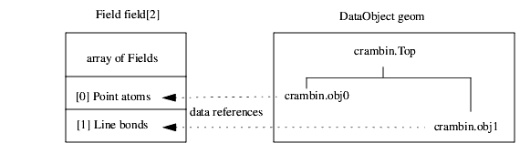
The V pre-processor symbols ACKIT or AC_KIT_V1 must be defined for the loading of v/modules.v, in order to access the Read Geoms module. These symbols are usually defined in include/$MACHINE/config.h, and this file is included directly by v/modules.v.
read an image file and output an AVS/Express field
Read_Image reads an image file and converts it into an AVS/Express Field.
- A port to connect to a user interface object that contains the macro's widgets. By default, it is connected to the default user interface object in the application in which the macro is instanced. (This default connection is not drawn.)
- File browser. Selects the disk file to input and convert. The default search pattern is $XP_PATH<0>/data/image/*.
- Boolean indicating whether to invert the image about the x axis, that is, in the vertical direction.
- An integer value indicating the file format. A value of 0 causes the format to be determined from the file itself by looking at the id information in the header, or by using the filename extension. Other values indicate the format explicitly. The following image formats are currently supported:
WARNING: Use of this software for providing LZW capability for any purpose is not authorized unless user first enters into a license agreement with Unisys under U.S. Patent No. 4,558,302 and foreign counterparts. For information concering licensing, please contact:
Unisys Corporation
Welch Licensing Department - C1SW19
Township Line & Union Meeting Roads
P.O. Box 500
Blue Bell, PA 19422
Once you have entered into such a license agreement with Unisys Corp, runtime generation support for GIF and TIFF can be enabled in AVS/Express at no additional cost. Contact Advanced Visual Systems customer support for details.
- Support for additional image formats can be provided by creating new readers using available API calls (see Appendix A, Adding your own image readers and writers). To obtain a current list of the supported image types, you can open v/modules.v and search for "Read_Image" - the list can be found in the defined radioBox labels.
- The output is a new Mesh_Unif object.
- Note: The order of the image's scan lines is reversed. For example, if an input image had four rows of pixels (0, 1, 2, 3) with 0 the "top" of the image, the output image has four rows of pixels (3, 2, 1, 0) with 0 at the "bottom" of the image. The reason for this is that the renderer recognizes 0,0 as the lower left of an object, not the upper left. Reversing the image's scan lines makes the image appear upright in the renderer window.
- Because the scan lines are reversed, a few image processing functions may not produce the same result as they would if the image was right side up. To ensure correct results, use the flip input parameter.
- The new Mesh_Unif contains:
veclen equals 4 (alpha, red, green, blue)
id equals GD_RGB_DATA_ID
values array contains the ARGBs of all pixels
primitive data type DTYPE_BYTE
dims array equal to dims[0] = x; dims[1] = y
points array equal to: points[0] = 0.0
points[1] = 0.0
points[2] = (float) x - 1
points[3] = (float) y - 1
- obj. This is a renderable version of the output field.
v/modules.v
modules/rd_image.c
modules/image.hread a dataset from a netCDF file
Read_netCDF reads a dataset from a netCDF file into an AVS/Express field. If the netCDF file was written with the AVS/Express Write_netCDF module, then Read_netCDF outputs the same object that was written (a field or other AVS/Express object). If the file contains only a standard netCDF object, without AVS/Express header information, Read_netCDF produces an object containing the data elements of the netCDF file.
- A port to connect to a user interface object that contains the macro's widgets. By default, it is connected to the default user interface object in the application in which the macro is instanced. (This default connection is not drawn.)
- UIfileSB. The name of the netCDF file to read.
- Mesh+Node_Data. The output field.
- Renderable object corresponding to field.
read an AVS volume (.dat file) and output an AVS/Express field
Read_Volume reads an Application Visualization System volume format file (.dat suffix) and converts it into an AVS/Express Field_Unif.
- A port to connect to a user interface object that contains the macro's widgets. By default, it is connected to the default user interface object in the application in which the macro is instanced. (This default connection is not drawn.)
- File browser. Selects the disk file to input and convert. The default search pattern is $XP_PATH<0>/data/volume/*.dat.
- The input file is an AVS volume (.dat) format binary file such as the AVS write volume module produces.
- The output is a new Field_Unif object containing:
nnodes equal to the product of the dims array (X x Y x Z)
nnode_data equals 1 (one Data_Array component)
nvals equals nnodes
veclen equals 1
values array contains the scalar node values
primitive data type OM_TYPE_BYTE
dims array equal to dims[0] = x dim; dims[1] = y dim; dims[2] = z dim
points array equal to: points[0] = 0.0
points[1] = 0.0
points[2] = 0.0
points[3] = (float) x - 1.0
points[4] = (float) y - 1.0
points[5] = (float) z - 1.0
read an AVS UCD (.inp file) and output an AVS/Express field
Read_UCD reads an Application Visualization System UCD format file (.inp suffix) and converts it into an AVS/Express Field.
- A port to connect to a user interface object that contains the macro's widgets. By default, it is connected to the default user interface object in the application in which the macro is instanced. (This default connection is not drawn.)
- UIfileSB file browser. Selects the disk file to input and convert. The default search pattern is $XP_PATH<0>/data/ucd/*.inp.
- The input file is an AVS UCD (.inp) format binary or ASCII file such as the AVS write ucd module produces.
- Field. The output is a new Field object.
- The new Field contains:
- nnode_data (number of components) equal to the number of components associated with each node in the input. For example, (a, [b, c, d], e) would have nnode_data = 3.
- Note that Read_UCD ignores any mid-edge nodes, treating the cells as though they had only corner nodes.
- values array contains the data of this component
labels equal to that component's label; " " default
units equal to that component's units; " " default
min, max are not set. They are derived via the Data_Array function
primitive data type DTYPE_FLOATncell_sets equal to the total number of different cell types (hex, pyr, tet, and so on), present in the input file. There will be one Cell_Set per type.
One for each different cell type and different material id in the input (for example:
type tet material id 7, type tet material id 4, type hex material
id 4 yields the three Cell_Sets: Tet & 7, Tet & 4, Hex & 4)
ncells equal to the total number of cells of this type
cell_name equal to cell type (Point, Tri, Quad, Tet, Hex, and so on)
remainder appropriate for that cell type
nnodes equal to the total number of nodes
nspace = 3
coordinates array equal to the input
min_vec and max_vec equal to input's min_ext, max_ext
- This is a renderable version of the output field.
Libraries.Examples.Visualization.Advect
examples/advect.v
Libraries.Examples.Visualization.Curl
examples/curl.vreset the transformation on a field to an identity
reset_xform resets the transformation of a field's mesh to be equal to an identity transformation. It is used to "desynchronize" the orientation of two fields.
- The input is any mesh. This is the field to transform.
- The output is a reference to an object that is the merge of the input mesh with the new transformation set.
- This is a renderable version of the output field.
Libraries.Examples.Visualization.Iso_Trace
examples/isotrc.vcreate "height surfaces" of a 2D field that are continuous along one axis but discontinuous along the other
ribbons_plot creates height surfaces of a 2D field by treating the values of a component of that field as height above the surface of the field, and the values of another component as color to be applied. The surfaces so created are continuous along one axis (selectable as X or Y) and discontinuous along the other axis, so they look like a set of colored ribbons draping over a surface. Each quadrilateral polygon composing a ribbon segment is created as follows:
Two points above a pair of node points along the continuous axis define the left side of the polygon. The polygon is flat (horizontal) along the other axis. The width of the ribbons is scaled by the scale slider, and the offset value is added to their height. Note that the ribbons, in general, extend one grid cell width past the grid in the +X and +Y directions, as shown above.
- Mesh_Unif+Node_Data. The ribbon plot is built on this mesh, using the node data values as heights.
- A port to connect to a user interface object that contains the macro's widgets. By default, it is connected to the default user interface object in the application in which the macro is instanced. (This default connection is not drawn.)
- UIradioBoxLabel. Selects which direction the ribbons should run.
- UIradioBoxLabel. Which node data component to map to ribbon height.
- UIradioBoxLabel. Which node data component to map to ribbon color.
- UIslider. This scale factor is applied to the data values to convert them into heights above the mesh.
- UIslider. This offset is added to the heights to offset the ribbons from the surface of the field.
- Mesh+Node_Data. The mesh contains the ribbons, with the node data containing the color.
- Renderable object corresponding to out_fld.
Libraries.Examples.Visualization.Ribbon_Plot
examples/rib_plot.vextract one or more Cell_Sets from a Cells Grid
select_cells extracts one or more Cell_Sets from a Cells Grid. For example, you use it if the Grid contains both Tri and Hex cells and all you want the downstream module to work on is the Tri cell_set.
- The input is a field with an unstructured Mesh. Typically, this mesh contains more than the usual one Cell_Set.
- A port to connect to a user interface object that contains the macro's widgets. By default, it is connected to the default user interface object in the application in which the macro is instanced. (This default connection is not drawn.)
- UIoptionBoxLabel. A series of buttons to select which Cell_Sets to extract. The labels displayed include the Cell_Set's cell_name value (the type of cell), plus any user-supplied names that may have been added. You can pick multiple Cell_Sets.
- The output is a reference to a merged object that contains a new Cells object with the selected cell_sets, plus the remainder of the input Mesh.
- This is a renderable version of the output field.
Libraries.Examples.Visualization.Cell_Data
examples/celld.vscale a 3D mesh in X, Y, and/or Z
scale scales a mesh in the X, Y, and/or Z direction, making it appear larger or smaller in the renderer window. The grid is unchanged, but its associated xform transformation matrix is altered.
- The input is any mesh. Any Node_Data that is present is ignored.
- A port to connect to a user interface object that contains the macro's widgets. By default, it is connected to the default user interface object in the application in which the macro is instanced. (This default connection is not drawn.)
- UIsliders. Floats. These inputs independently control the degree of X, Y, and Z scaling. The default is 1.0 (leave at current size). The range is -10.0 to 10.0.
- The output field is the same mesh as the input mesh, but with its xform matrix changed to reflect the scaling.
- This is a renderable version of the output field.
Libraries.Examples.Visualization.Mirror_Scale
examples/mirr_scl.vconverts a scattered grid into triangular or tetrahedral unstructured mesh
scat_to_tri converts a field with a scattered grid into a triangular or tetrahedral mesh. A "scattered grid" means that there is a mesh made up of disconnected nodes in space. An example is seismic data, where the coordinates are the latitude, longitude, (and perhaps elevation) of a sensing station, and the Node_Data was a set of observations. The grid is "scattered" because there is not data for every latitude, longitude, and elevation that exists.
Fields whose meshes have nspace=2 are converted to triangular unstructured meshes. For meshes having nspace=3, if the 2D(triangles) toggle is off, they are converted to tetrahedral unstructured meshes; if the 2D(triangles) toggle is on, they are converted to a triangular unstructured mesh (a surface existing in 3-space).
- The input is a field with any mesh. If Node_Data is present, a reference to it is copied to the output field.
- A port to connect to a user interface object that contains the macro's widgets. By default, it is connected to the default user interface object in the application in which the macro is instanced. (This default connection is not drawn.)
- UItoggle. This toggle only has meaning if the input is nspace=3. If off, the scattered grid is converted to a tetrahedral unstructured mesh (essentially a three-dimensional volume existing in 3-space. If on, the scattered grid is converted to a triangular unstructured mesh (essentially a two-dimensional surface existing in 3-space). The default is off.
- The output is a new unstructured mesh with cell type Tri (for nspace=2 or nspace=3 with 2D toggle on input) or Tet (nspace =3 input). If Node_Data was present in the input field, the output field contains a reference to it.
- This is a renderable version of the output field.
scat_to_tri uses a proprietary version of the Delaunay tessellation algorithm.
Libraries.Examples.Visualization.Scat_to_Tet
examples/sct2tet.vinterpolate scattered data into a uniform mesh
scat_to_unif converts a field with a scattered grid into a field with a uniform mesh. A "scattered grid" has a structured mesh made up of disconnected nodes in space. An example is seismic data where the coordinates are the latitude, longitude, and perhaps elevation, of a sensing station, and the Node_Data is a set of observations. The grid is "scattered" because there is not data for every latitude, longitude, and elevation that exists.
scat_to_unif lets you define a uniform mesh of any dimensionality, coordinate extents, and physical extents. It superimposes the input grid over this new grid that you defined. Then, it searches the input grid's neighboring real nodes that have data (where search distance X, Y and Z control what is a neighbor), and creates data values for all the nodes in the new grid by interpolating from those neighboring data values. You can control the order of interpolation, what values are considered NULL, and what number to use as the NULL data value.
- The input is a field with any mesh and Node_Data.
- A port to connect to a user interface object that contains the macro's widgets. By default, it is connected to the default user interface object in the application in which the macro is instanced. (This default connection is not drawn.)
- UIradioBoxLabel. Radio buttons to pick which component to use for the data generation. The selection can be scalar or vector. The default is the first (0th) component. If node data labels are present, they are displayed.
- UIslider. Sets the dimensionality of the "search cube", "search rectangle", or "search line" that is used to traverse the data. The default is 3 (search cube). The range is 1 to 3.
- UIsliders. Set the dimensions of the search cube, rectangle, or line (depending on the input dimensionality). Use as many as necessary to match ndim. The defaults are 10 for each. Their range is 0 to 1000.
- UIsliders. Float. Set the depth of the search for nodes in the input mesh. The defaults are (max_xyz - min_xyz)/10.
- UIslider. Integer. Controls the order of interpolation performed on the adjacent nodes. The default is 2. The range is 0 to 32.
- The output is a uniform mesh (mesh type Mesh_Unif). Its Node_Data is the interpolated data values at each node in the uniform grid.
- This is a renderable version of the output field.
Libraries.Examples.Visualization.Scat_to_Unif
examples/sct_unif.vflag a specified data value as NULL or not NULL in one component of a field
set_null alters a field by defining a specified value as a NULL value and setting the flag that indicates the presence of NULL data to 1 ("has null data"). This is done on a per-component basis-one component may have NULL data while others do not.
set_null can also unset the flag that indicates NULL data.
- The input must contain Node_Data.
- A port to connect to a user interface object that contains the macro's widgets. By default, it is connected to the default user interface object in the application in which the macro is instanced. (This default connection is not drawn.)
- UIradioBoxLabel. Radio buttons to pick which component will be flagged as having NULL data (or to unflag). The components can be scalar or vector. The default is the first (0th) component. If node data labels are present, they are displayed.
- UIfieldTypein. A float typein. Specifies the data value that is treated as a NULL value. The default is 0.
- UItoggle. Unflag data component as having NULL data. The default is off.
- The output is a reference to the input field. The input field's Node_Data has been altered so that the null_flag =1 and null_value is set for the component's Data_Array. set_null is one of the few macros that actually changes its input data field.
- If unset was toggled, null_flag=0.
- This is a renderable version of the output field. (The field is renderable only if it included a mesh.)
Libraries.Examples.Visualization.Null_Data
examples/nulldt.vset the transformation on a field
set_xform sets the transformation of a field's mesh to equal that of another input transformation. It is used when you want to "synch up" the transformation of one field with another.
- The input is any mesh. This is the field to transform.
- The input is any field with a Grid. This Grid's transformation (xform) is used to transform in_field1.
- The output is a reference to an object that is the merge of the input mesh with the new transformation set.
- This is a renderable version of the output field.
Libraries.Examples.Visualization.Iso_Trace
examples/isotrc.vproduce a mesh with cells shrunk relative to their geometric centers
The shrink_cells module produces a mesh containing disjoint cells which can be optionally shrunk relative to their geometric centers. It creates duplicate nodes for all cells that share the same node, making them disjoint. If the shrink cells toggle is set, the module computes new coordinates for the nodes based on the specified shrink factor (which specifies the scale relative to the geometric centers of each cell). The shrink factor can vary from 0 to 1. A value of 0 produces non-shrunk cells; 1 produces completely collapsed cells (points). This module is useful for separate viewing of cells comprising a mesh.
- The input must contain any type of mesh.
- A port to connect to a user interface object that contains the macro's widgets. By default, it is connected to the default user interface object in the application in which the macro is instanced. (This default connection is not drawn.)
- UItoggle. If off, the output mesh will contain disjoint cells with the same coordinates as the input mesh. If set on, the module computes new coordinates for the nodes based on the shrink factor that specifies the scale relative to the geometric centers of each cell. The default is on.
- UIslider. A float slider to adjust the sizes of the cells. The shrink factor value specifies the scale relative to the geometric centers of each cell. The shrink factor value can vary from 0 to 1, 0 producing non-shrunk cells and 1 producing completely collapsed cells (points). The default is 0.3. The range is 0.0 to 1.0.
- The output field contains a new mesh that contains disjoint cells shrunk relative to their geometric centers. It also contains a Node_Data and Cell_Data if present in the input mesh.
- This is a renderable version of the output field.
Libraries.Examples.Visualization.Shrink_Cells
examples/shrink.vextract a 2D slice from a field with an arbitrarily positioned slice plane
slice extracts an arbitrarily-oriented 2D slice of data from a 3D (or 2D) mesh field. Output is generated every time the slice plane moves.
- The input is any 3D or 2D mesh. It may optionaly have node and/or cell data that can be mapped onto resulting mesh.
- The slicing plane. This is a 2D Mesh_Unif. It is generated by the plane object found in Geometries.FPlane or Geometries.Plane. The plane object has its own Plane Transformation panel that controls plane rotation, translation, and scale, as well as controls to specify its size when it is connected to the default user interface object in the application in which the macro is instanced.
- A port to connect to a user interface object that contains the macro's widgets. By default, it is connected to the default user interface object in the application in which the macro is instanced. (This default connection is not drawn.)
- UIoptionBoxLabel. Option buttons to pick which components of in_field's node data to map to the output field. The default is the first (0th) component. If node data labels are present, they are displayed.
- UIoptionBoxLabel. Option buttons to pick which components of in_field's cell data to map to the output field. The default is the first (0th) component. If cell data labels are present, they are displayed.
- UIslider. A float slider that moves the plane through the field perpendicular to the plane's current orientation. Though the Plane Transformation panel has X, Y, and Z transformation controls, it is usually easier to use plane's controls to orient and size the plane, but use this plane distance control to move the plane. slice generates output whenever the slice plane moves.
- The default distance is 0.0. The minimum range is the (absolute value of maximum coordinate - minimum coordinate) * -0.5. The maximum range is the (absolute value of the maximum coordinate - minimum coordinate) * 0.5.
- The output field contains a new, subsetted 2D (or 1D) mesh and a new node and/or cell data.
- This is a renderable version of the output field.
The interpolation algorithm for calculating coordinates and node data values is trilinear for structured meshes, and shape functions for unstructured meshes.
Libraries.Examples.Visualization.Slice
examples/slice.v
Libraries.Examples.Visualization.Threshold
examples/thresh.v
Libraries.Examples.Visualization.Clamp
examples/clamp.vextract a 2D slice from a field with an arbitrarily positioned slice plane
slice_plane is a macro that contains the slice macro and a slicing plane object. It extracts a 2D or 1D slice from a 3D or a 2D field at a given distance from the plane. See the documentation for the slice macro for details.
- Mesh. The field to slice, which can be any 3D or 2D mesh.
- A port to connect to a user interface object that contains the macro's widgets. By default, it is connected to the default user interface object in the application in which the macro is instanced. (This default connection is not drawn.)
- UIoptionBoxLabel. Option buttons to pick which components of in_field's node data to map to the output field. The default is the first (0th) component. If node data labels are present, they are displayed.
- UIoptionBoxLabel. Option buttons to pick which components of in_field's cell data to map to the output field. The default is the first (0th) component. If cell data labels are present, they are displayed.
- UIslider. A float slider that moves the plane through the field perpendicular to the plane's current orientation. Though the Plane Transformation panel has X, Y, and Z transformation controls, it is usually easier to use plane's controls to orient and size the plane, but use this plane distance control to move the plane. slice generates output whenever the slice plane moves.
- The default distance is 0.0. The minimum range is the (absolute value of maximum coordinate - minimum coordinate) * -0.5. The maximum range is the (absolute value of the maximum coordinate - minimum coordinate) * 0.5.
- The output field contains a new, subsetted 2D (or 1D) mesh and a new node and/or cell data.
- Plane_Mesh. A 2D mesh representing the plane used to do the slicing.
- Renderable object corresponding to out_fld.
- Renderable object corresponding to out_plane. This may be fed to the viewer and transformed to transform the slicing plane.
create a 2D texture mapped slice of a uniform field
slice_texture2D uses a 2D slice plane to extract a slice from a 3D uniform field. It then 2D texture maps this slice plane with colors representing the data values of the first component (which must be scalar) on the extracted slice.
- The input is a Mesh_Unif with Node_Data, The first component is used to create the texture map.
- The slicing plane. This is generated by the plane object found in Geometries.Plane or Geometries.FPlane. The plane object has its own Plane Transformation panel that controls plane rotation, translation, and scale, as well as controls to specify its size when it is connected to the default user interface object in the application in which the macro is instanced.
- A colormap to provide the texture map, from Libraries.Main.Fields.Data.colormap.
- The output is a 2D Mesh_Unif. Its Node_Data is the u, v, w texture mapping values. Its points array (extents) is set to retain the position of the field in space.
- This is a renderable version of the output field.
Libraries.Examples.Visualization.Slice_Texture2D
examples/slc_txt2.vcreate a 3D texture mapped slice of a uniform field
slice_texture3D uses a slicing object to extract a plane of data from a 3D uniform field. It then 3D texture maps the surface of this plane with colors representing the data values of the first component (which must be scalar) on the extracted surface.
- The input is a Mesh_Unif with Node_Data. The first component's value is used to create the texture map.
- The slicing plane. This is generated by the plane object found in Geometries.Plane or Geometries.FPlane. The plane object has its own Plane Transformation panel that controls plane rotation, translation, and scale, as well as controls to specify its size when it is connected to the default user interface object in the application in which the macro is instanced.
- A colormap to provide the texture map, from Libraries.Main.Fields.Data.colormap.
- The output is a 3D Mesh_Unif. Its Node_Data is the u, v, w texture mapping values. Its points array (extents) is set to retain the position of the volume of the field in space.
- This is a renderable version of the output field.
Libraries.Examples.Visualization.Slice_Texture3D
examples/slc_txt3.vcreate multiple 2D or 3D filled contours
solid_contour produces solid (filled) contour regions of a given component of an input field. If the input mesh is 2D, the output is similar to contour lines, except the regions between the lines are filled with a color representing the value of that contour. The output cells are subdivisions of the input cells, cut by the contour lines.
If the input mesh is 3D, the output is a set of 3D cells filling the regions between adjacent isosurfaces. The output cells are, in general, subdivisions of the input cells, cut by the contour surfaces.
The number of contour regions is set by the parameters; the region boundaries are evenly spaced from level_min to level_max. The data value in the output cells is the average of the values of the two contour lines or surfaces bounding that region.
- Note: The solid_contour module does not generate vertex normals by default. For more details, see Section 5.1.8, Vertex normal generation [page 5-4].
- Mesh+Node_Data. 2D or 3D input field to contour.
- A port to connect to a user interface object that contains the macro's widgets. By default, it is connected to the default user interface object in the application in which the macro is instanced. (This default connection is not drawn.)
- UIradioBoxLabel. Select which component of in_field to contour.
- UIslider. Sets the number of contour regions.
- UIslider. Sets the lowest contour level.
- UIslider. Sets the highest contour level.
- Mesh+Cell_Data. Represents the solid contours. This mesh has the same dimensionality as the input.
- Renderable object corresponding to out_fld.
Libraries.Examples.Visualization.Solid_Contour
examples/sol_con.vintegrate a velocity field producing streamlines or streamribbons
streamlines generates streamlines or streamribbons based on a field of any mesh type that has at least one component that is a one-, two-, or three-element vector.
You place a sample of points (the in_probe) at a starting location in the field. Then, for every time step, streamlines advances each sample point through space based on the interpolated value of the vector field at its present position. The result is a set of streamlines or streamribbons showing the progress of massless particles through a vector field.
streamlines is similar to the advector macro, except that the result is a set of lines instead of a dynamically updated set of glyphs.
- The input field can have any type of mesh. Its Node_Data must contain at least one component that is a one-, two-, or three-element velocity vector.
- Any mesh whose coordinates represent the sample points. To create this sampling mesh you can use the plane objects in Geometries or the slice macro.
- A port to connect to a user interface object that contains the macro's widgets. By default, it is connected to the default user interface object in the application in which the macro is instanced. (This default connection is not drawn.)
- UIradioBoxLabel. Radio buttons to pick on which component to base the streamlines. The selection must be a three-element vector.
- UIradioBoxLabel. Radio buttons to pick the direction of streamline generation, forward or backward. The default is forward.
- UIslider. An integer slider that sets how many integration steps will be used within one grid "cell" to compute the streamline path. The default is 2. The range is from 0 to 16.
- UIslider. An integer slider that sets the total number of integration steps. When an individual streamline exceeds this value, integration for it stops. The range is from 1 to 10000. The default is 256.
- UIslider. An integer slider that sets the order of integration. Higher orders are more accurate, but execute more slowly. The default is 2. The range is from 1 to 4.
- UIslider. A float slider. When a streamline falls below this velocity, the integration process for that streamline stops. The default is 0.00001. The range is from 0.0 to unbounded. You can use this to prevent wasted computation for streamlines barely moving, or even stationary (min_velocity = 0).
- UItoggle. When on, streamlines produce streamribbons rather than streamlines. The default is off.
- UIslider. An integer slider. Scales the width of the ribbon. Ribbon width varies along its length according to the divergence of the flow. This value controls ribbon width at the beginning of the ribbon. The default is 1. The range is unbounded.
- UIslider. An integer slider. Controls the initial angle at which the ribbon is drawn. The default is 0. The range is 0.0 to 360.0.
- The output field is a new unstructured mesh of cell type Polyline that represents the streamlines. Its new Node_Data contains the selected element's velocity component. The output also contains a reference to the input field's xform.
- This is a renderable version of the output field.
The streamlines are calculated using the Runge-Kutta method of specified order with adaptive time steps.
Libraries.Examples.Visualization.Stream
examples/stream.vcreate streamlines and stream ribbons for a Multi_Block object
stream_multi_block creates streamlines and stream ribbons for a Multi_Block object.
- Multi_Block. The input multiblock dataset.
- Plane_Mesh. Streamlines start at each node of this mesh.
- A port to connect to a user interface object that contains the macro's widgets. By default, it is connected to the default user interface object in the application in which the macro is instanced.
- UIradioBoxLabel. When on (nonzero), streamlines are advected forward, in the downstream direction of the flow. When off (zero), they are advected backward, upstream in the flow. The default is forward.
- UIslider. The number of integration steps used per grid cell to compute the streamline path. The default is 2.
- UIslider. Maximum number of integration steps to take for an individual streamline. A streamline is terminated either when it leaves the dataset, when the absolute value of its velocity is less than the min_velocity parameter, or when it exceeds this number of integration steps.
- UIslider. Integration order for the streamline advection. Higher orders are more accurate but execute more slowly. The default is 2, for second-order integration. The range is from 1 to 4.
- UIslider. If the absolute value of the velocity is less than this limit, the streamline advection is terminated. This is usually used to avoid wasting computation on streamlines which are barely moving. Velocity is measured in the coordinate system of the dataset. The default is 0.000001.
- UItoggle. When on (nonzero), color the streamlines by velocity. When off (zero), do not color the streamlines. Default is on.
- UItoggle. When on (nonzero), stream_multi_block produces stream ribbons rather than streamlines. The width of the ribbons varies along the length with the divergence of the field, and the angle varies with the curl.
- UIslider. This value scales the width of the ribbons when Ribbons are turned on.
- UIslider. This value sets the initial angle at which the ribbons are drawn. The ribbons twist along their length according to the curl of the field.
- Mesh+Node_Data. Field containing the streamlines.
- Renderable object corresponding to out_fld.
Libraries.Examples.Visualization.Multi_Block
examples/mblock.vproduce an optimized (in terms of biggest possible triangles) triangular mesh from a 2D uniform elevation data field
The surf_optimize module is used to optimize 2D uniform meshes with a scalar node data component. The node data is assumed to be an elevation (height) at each grid point. This type of mesh is typically used in GIS applications where it is called a Digital Elevation Model (DEM). To find out more about AVS/Express GIS functionality, see Chapter 6, Geographic Information System (GIS) Components.
The module creates a mesh containing "optimum" triangles. In this usage, the term "optimum" means that the largest possible triangles that satisfy a specified tolerance criteria are met. The tolerance determines the maximum difference of elevations between any point in the output triangular mesh and the corresponding point of the input mesh. That is, the output surface of the elevation lies within the specified tolerance from original surface of elevation.
This module is used to create a coarse mesh in the regions where the surface of elevation changes gradually and a fine mesh in the regions where the surface changes rapidly. Increasing the tolerance results in a less accurate mesh containing fewer triangles and thus leads to a corresponding improvement in rendering performance. The surf_optimize module does not produce the elevation surface itself, it just creates a flat triangular mesh that can be extruded into a surface of elevation produced using the surf_plot module (see page 5-240). The algorithm used in this module is described in: Automatic Generation of Triangular Irregular Networks using Greedy Cuts by Claudio T. Silva, Joseph S. B. Mitchell and Arie Kaufman, Visualization 95 Proceedings.
- The input must contain a 2D uniform mesh with a scalar node data.
- A port to connect to a user interface object that contains the macro's widgets. By default, it is connected to the default user interface object in the application in which the macro is instanced. (This default connection is not drawn.)
- UIslider. A float slider to adjust the accuracy of the output mesh and the number of triangles generated. Increasing tolerance results in a less accurate mesh containing fewer triangles and thus leads to a corresponding improvement in rendering performance. The default is 10% of the difference between the max and min elevation values.
- The output field contains a triangular mesh with a elevation node data.
- A renderable version of the output field.
Libraries.Examples.Visualization.Surface_Optimize
examples/surf_opt.vproduce a 3D or 2D surface by extruding 2D|1D mesh according to data values
surf_plot creates a 3D or 2D mesh whose height at each point is proportional to the scalar data value at that node location in the original field. 2D input produces a 3D mesh. 1D input produces a 2D output.
- The input is a field of any mesh type and any Node_Data. The field's mesh must have nspace=1 or 2. However, no checking is done to enforce this restriction. (Inputting an nspace=3 mesh will not generate a picture.) The Node_Data must contain at least one scalar component.
- A port to connect to a user interface object that contains the macro's widgets. By default, it is connected to the default user interface object in the application in which the macro is instanced. (This default connection is not drawn.)
- UIradioBoxLabel. Radio buttons to pick which of the input's data components to use to set the mesh height. The default is the first (0th) component. You must select a scalar component. If node data labels are present, they are displayed.
- UIslider. A float slider to scale the height (scale*component values). The default is 1.0. The range is -10.0 to 10.0.
- UIslider. A float slider that raises or lowers the resulting mesh with respect to the input mesh. The default is 0.0. The range is unbounded.
- The output is a mesh of the same type as the input mesh, with nspace+1, whose coordinate values represent the projected, scaled, and offset surface. Its Node_Data contains the data in the selected component.
- This is a renderable version of the output field.
Libraries.Examples.Visualization.Surf_plot
examples/splot.vmaps the data in an array of DBcolumn to a scattered field.
Table_to_Scattered_Field maps the data in an array of DBcolumn to a 1D, 2D, or 3D scattered field (an unstructured field that can store scattered data). The data to be mapped is usually query data returned by DBquery or Query.
You typically use scattered fields to represent sparse data, whose columns have many missing values, or nonconnected data, in which there are no internal logical connections between database records. When mapping query data to a scattered field, each record is viewed as a separate point that may have several data values associated with it.
You can visualize scattered field data directly using glyph modules. Alternatively, you can map it to the an unstructured field type using a triangulation process (or, in 3D, a tetrahedration process). After mapping it, you can apply most AVS/Express visualization techniques to the results; for example, isosurface, slice, or surface_plot. This type of visualization is suitable mainly for cluster analysis.
Table_to_Scattered_Field provides a number of parameter values that control various aspects of the mapping.
You use the X Axis, Y Axis, and Z Axis selection menus to select one, two, or three columns that will serve as the coordinate axes of the resulting scattered field. The number of spatial dimensions in the output field will be one, two, or three, respectively. You use the On toggle associated with each menu to turn the corresponding axis on.
You use the Axis Setup menu to specify a column whose axis parameter you want to set. This parameter value is used when you select the column as a coordinate axis. The Discrete parameter is available. It specifies whether the coordinates along an axis are discrete or continuous.
- If you select Discrete, discrete coordinates are used. They are the indices of the rows in a column, rather than the rows' values. Note that every row is assigned its own index value, including duplicate row values. (By comparison, Table_to_Uniform_Field uses only unique values.)
- Discrete coordinates are particularly useful with numeric data such as area codes or with string values. For example, if the column contains the string values "John", "Bob", "Bob", "John", "Bill", the coordinates are 0, 1, 1, 0, and 2, where 0 represents "John", 1 represents "Bob", and 2 represents "Bill".
- If you deselect Discrete, continuous coordinates are used; that is, each value in the column is treated as a separate coordinate value.
- Note: Continuous coordinates cannot be used with string values.
You use the Field Data selection menu to select the columns that will become data components in the resulting scattered field. You use Data Setup to specify a column whose data parameter you want to set. This parameter value is used when you select the column using Field Data.
The data parameter sphere radius is available. Selecting sphere radius for a particular column puts its data components into a field with a special ID. When visualized, the renderer treats this data as sphere radii.
- An array of type DBcolumn that contains the query data returned by a SELECT statement. This is the output of a DBquery module or Query macro.
- The UI parent, of type UIconnection.
- A menu from which you can choose the name of a column that will serve as the X coordinate axis. The possible values are the names of the columns in the columns[] input por
- A toggle, located to the right of the X Axis menu, that turns on or off the X coordinate axis. The default is on.
- A menu from which you can choose the name of a column that will serve as the Y coordinate axis. The possible values are the names of the columns in the columns[] input port.
- A toggle, located to the right of the Y Axis menu, that turns on or off the X coordinate axis. The default is off.
- A menu from which you can choose the name of a column that will serve as the Z coordinate axis. The possible values are the names of the columns in the columns[] input port.
- A toggle, located to the right of the Z Axis menu, that turns on or off the X coordinate axis. The default is off.
- A menu from which you can choose the name of a column whose axis parameter you want to set. This parameter value is used when you select the column as a coordinate axis.The possible values are the names of the columns in the columns[] input port.
- A toggle that specifies whether to use discrete or continuous coordinates on the axes. If selected (the default), discrete coordinates are used, otherwise continuous coordinates are used.
- Note: Continuous coordinates cannot be used with string values.
- A menu from which you can choose the columns that will become data components in the output scattered field. The first possible value is Count Records (see next parameter description); the other possible values are the names of the columns in the columns[] input port.
- A menu from which you can choose the name of a column whose field data parameter you want to set. This parameter value is used when you select the column using Field Data. The possible values are the names of the columns in the columns[] input port.
- A toggle that specifies whether the data in a column should be treated as sphere radii. If selected (the default), the data values in the column specified with Data Setup are put into a field with a special ID, and when visualized, the renderer treats the data as sphere radii.
- A scattered field with its data.
- A renderable field.
- The name of the column selected as the X coordinate axis.
- The name of the column selected as the Y coordinate axis.
- The name of the column selected as the Z coordinate axis.
maps the data in an array of DBcolumn to a uniform field.
Table_to_Uniform_Field maps the data in an array of DBcolumn to a 1D, 2D, or 3D uniform field. The data to be mapped is usually query data returned by DBquery or Query.
You typically use uniform fields to represent regular data whose records form continuous 1D, 2D, or 3D uniformly spaced arrays. You can visualize a uniform field in many ways; for example, city_plot, ribbon_plot, surface_plot, contour, isosurface, or isoline.
Table_to_Uniform_Field provides a number of parameter values that control various aspects of the mapping.
You use the X Axis, Y Axis, and Z Axis selection menus to select one, two, or three columns that will serve as the coordinate axes of the resulting uniform field. The number of dimensions in the output field will be one, two, or three, respectively. You use the On toggle associated with each menu to turn on the corresponding axis.
You use the Axis Setup menu to specify a column whose axis parameters you want to set. These parameter values are used when you select the column as a coordinate axis. The following axis parameters are available:
The Discrete parameter specifies whether the coordinates along an axis are discrete or continuous.
- If you select Discrete, discrete coordinates are used. They are the indices of an array of the unique values in a column. For example, a column that contains the values 1, 2, 3, 2, 3, 2, 10, and 20 has five unique values (1, 2, 3, 10, and 20) and therefore five indices: 0, 1, 2, 3, and 4. These indices serve as the discrete coordinates.
- Discrete coordinates are particularly useful with numeric data such as area codes or with string values. For example, if a column contains the string values "John", "Bob", "Bob", "John", "Bill", the coordinates are 0, 1, and 2, where 0 is the index of "John", 1 is the index of "Bob", and 2 is the index of "Bill".
- With discrete coordinates, the dimensionality of the coordinate array is always the number of unique values in the column.
- If you deselect Discrete, continuous coordinates are used. They are calculated based on the values that you supply for the Min value, Max value, and Bin size parameters. The dimensionality of the coordinate array is the number of bins between Min value and Max value, and the value of the coordinates are the centers of consecutive bins.
- Suppose that the values of Min value, Max value, and Bin size are 0.00, 4.00, and 1.00, respectively. The following figure illustrates how the coordinates are calculated:
- With parameter values as noted, there are four bins from Min value to Max value, and the coordinates are 0.50, 1.50, 2.50, and 3.50.
- With continuous coordinates, the data values input to Table_to_Uniform_Field are binned; that is, they are put into the bins thus created. Data values that fall on a bin boundary are put into the immediately lower bin. In the previous figure, for example, a data value of 2.00 is put into the bin whose coordinate is 1.50. The data values in each bin are the sum or average of all of the values that fall into the bin, as specified with the field data parameters sum and average.
- Note: Continuous coordinates cannot be used with string values.
You can normalize the value of both discrete and continuous coordinates to the range [0,1] by setting the normalize axis toggle to on.
You can use the set label toggle to cause Table_to_Uniform_Field to output a string of labels that can be used by Axis modules.
The index labels toggle produces labels that are indices of coordinates rather than real numbers. This is useful when binning data. For example, when binning days into months, the axis labels should reflect the indices of the bins (month) rather than original values (days).
The label step slider bar allows you to control the frequency with which labels are applied to the coordinates on an axis. For example, if you select 3, a label is applied to every third coordinate.
You use the Field Data selection menu to select the columns that will become node data components in the resulting uniform field.
Optionally, you can use the Count Records toggle in the Field Data menu to count the number of values in a bin. If you select Count Records, the first data component of the field is a value that represents the number of records in each bin. As noted previously, for the rest of the columns, the data values in each bin are the sum or average of all of the values that fall into the bin, as specified with the field data parameters sum and average.
You use the Data Setup menu to specify a column whose data parameters you want to set. These parameter values are used when you select the column using Field Data. The data parameters sum and average are available as items in a radio box: sum causes the data in each bin to be summed, while average causes the data to be averaged.
- An array of type DBcolumn that contains the query data returned by a SELECT statement. This is the output of a DBquery module or Query macro.
- The UI parent, of type UIconnection.
- A menu from which you can choose the name of a column that will serve as the X coordinate axis. The possible values are the names of the columns in the columns[] input port.
- A toggle, located to the right of the X Axis menu, that turns on or off the X coordinate axis. The default is on.
- A menu from which you can choose the name of a column that will serve as the Y coordinate axis. The possible values are the names of the columns in the columns[] input port.
- A toggle, located to the right of the Y Axis menu, that turns on or off the X coordinate axis. The default is off.
- A menu from which you can choose the name of a column that will serve as the Z coordinate axis. The possible values are the names of the columns in the columns[] input port.
- A toggle, located to the right of the Z Axis menu, that turns on or off the X coordinate axis. The default is off.
- A menu from which you can choose the name of a column whose axis parameters you want to set. These parameter values are used when you select the column as a coordinate axis.The possible values are the names of the columns in the columns[] input port.
- A toggle that specifies whether to use discrete or continuous coordinates on the axes. If selected (the default), discrete coordinates are used, otherwise continuous coordinates are used.
- Note: Continuous coordinates cannot be used with string values.
- For continuous coordinates, a field in which you specify a floating-point value that specifies the lowest value used in calculating coordinates. The default is the lowest data value in the column. Min value should be less than Max value.
- For continuous coordinates, a field in which you specify a floating-point value that specifies the highest value used in calculating coordinates. The default is the highest data value in the column. Max value should be greater than Min value.
- For continuous coordinates, a field in which you specify a floating-point value that specifies the size of the bins into which the axis is divided. The default is 1.00.
- A toggle that specifies whether to normalize the value of coordinates to the range [0, 1]. If selected (the default), the values are normalized.
- A toggle that causes Table_to_Uniform_Field to output an array of label strings that can be used by Axis modules. If selected (the default), the labels are produced.
- A toggle that produces labels that are indices of coordinates rather than real numbers. If selected (the default), the labels are produced.
- This parameter is relevant only if you have also selected set labels.
- A slider bar that specifies the frequency with which labels are applied to the coordinates on an axis. For a value of n, a label is applied to every nth coordinate.
- This parameter is relevant only if you have also selected set labels.
- A menu from which you can choose the columns that will become data components in the output uniform field. The first possible value is Count Records (see next parameter description); the other possible values are the names of the columns in the columns[] input port.
- A toggle that causes the module to count the number of values in a bin. If selected (the default), the following happens:
- The first data component of the field is a value that represents the number of records in each bin.
- For the rest of the columns, the data values in each bin are calculated by an averaging or a summation of all of the values that fall into a particular bin, as specified by the sum and average parameters.
- A menu from which you can choose the name of a column whose field data parameters (sum and average) you want to set. These parameter values are used when you select the column using Field Data.The possible values are the names of the columns in the columns[] input port.
- Radio box items that specify how the data values in a bin are calculated. When you select sum (the default), the values are summed; otherwise the values are averaged. These parameters are mutually exclusive.
- A uniform field with its data.
- A renderable field.
- Labels for the X, Y, and Z axes.
- The name of the column selected as the X coordinate axis.
- The name of the column selected as the Y coordinate axis.
- The name of the column selected as the Z coordinate axis.
display a text string at the coordinates in the input mesh
text_glyph takes a Mesh and an array of strings and displays a string at each coordinate in the Mesh.
- The input field. The coordinates in the field are used as position at which to display the text strings.
- The input array of strings. A string is displayed at each coordinate in the input mesh. If not enough strings exist, the module cycles through the array of strings.
- Graphics Display Kit DefaultObject. This is a renderable object that can be connected directly to one of the Graphics Display Kit's viewers.
Libraries.Examples.Visualization.Text_Glyph
map an image onto a surface, using UV coordinates generated from the surface XY coordinates
texture_mesh uses the texture facility of the viewer to map an image onto a surface. The texture is applied using the (X,Y) coordinates of the mesh, so that the whole image is mapped to the (X,Y) range of the mesh. By default, the lower left of the texture is applied and xmin, ymin, and the upper right is applied at xmax, ymax. See the parameters for how to change this.
- Field. The mesh to texture.
- Field_Unif+Dim2+Space2. The image to texture onto in_field.
- A port to connect to a user interface object that contains the macro's widgets. By default, it is connected to the default user interface object in the application in which the macro is instanced. (This default connection is not drawn.)
- UItoggle. Switch U and V (or X and Y) when generating the texture coordinates.
- UItoggle. Flip U so that the texture is applied backwards in X.
- UItoggle. Flip V so that the texture is applied backwards in Y.
- UIslider. Scale U by this amount. The larger this value, the less space taken by the texture in X. Decreasing this value stretches the texture, increasing it compresses the texture.
- UIslider. Scale V by this amount. The larger this value, the less space taken by the texture in Y. Decreasing this value stretches the texture, increasing it compresses the texture.
- UIslider. Shift U by this amount. Positive shift shifts the texture to the left, negative shifts to the right.
- UIslider. Scale V by this amount. Positive shift shifts the texture down, negative shifts up.
- Mesh+Node_Data. Contains the input mesh with the texture applied.
- Renderable object corresponding to out_fld.
Libraries.Examples.Visualization.Texture_Mesh
examples/txt_mesh.vcreate a spher and map an image onto it
texture_sphere creates a sphere (or part of a sphere) with specified parameters and uses the texture facility of the viewer to map an image onto it.
- Field_Unif+Dim2+Space2. The image to texture onto in_field.
- A port to connect to a user interface object that contains the macro's widgets. By default, it is connected to the default user interface object in the application in which the macro is instanced. (This default connection is not drawn.)
- UIslider. Number of sub-divisions for sphere in the longitude direction. Default is 24.
- UIslider. Number of sub-divisions for sphere in the latitude direction. Default is 24.
- UIfield. Radius of a sphere, default is 6378000 (Earth).
- UIdial. Longitude in degrees of the begining of sphere segment. Default is 0.
- UIdial. Longitude in degrees of the end of sphere segment. Default is 360.
- UIdial. Latitude in degrees of the begining of sphere segment. Default is -90.
- UIdial. Latitude in degrees of the end of sphere segment. Default is 90.
- Mesh+Node_Data. Contains the spherical mesh with the texture applied.
- Renderable object corresponding to out_fld.
Libraries.Examples.Visualization.Texture_Sphere
examples/txt_sphr.vthreshold_cell sets the values of a given component of a cell-based dataset to the null value if the value of another component (usually the same one) is above or below a given threshold.
- Mesh+Cell_Data. The cell dataset to threshold.
- A port to connect to a user interface object that contains the macro's widgets. By default, it is connected to the default user interface object in the application in which the macro is instanced. (This default connection is not drawn.)
- UIradioBoxLabel. Selects which component to check. If this component exceeds the threshold(s) at some node, the value of the threshold_component at that node is set to the null data value.
- UIradioBoxLabel. Selects which component to threshold, based on the value of "check component."
- UItoggle. When set (nonzero), values below the selected min value are set to the null value.
- UIslider. The min value to check against.
- UItoggle. When set (nonzero), values above the selected max value are set to the null value.
- UIslider. The max value to check against.
- UIslider. The value to use in the output as the null value. Select a value for this which does not occur in the input dataset.
- Mesh+Cell_Data. Contains the thresholded data.
- Renderable object corresponding to out_fld.
remove cells with nodes that contain NULL data from input field
thresh_null removes cells where the selected component's node data is NULL. While the renderer automatically deletes NULL data cells, it must do so every time the object is transformed. You can remove this overhead using thresh_null as a data "preprocessor."
- The input field must contain any mesh and Node_Data.
- A port to connect to a user interface object that contains the macro's widgets. By default, it is connected to the default user interface object in the application in which the macro is instanced. (This default connection is not drawn.)
- UIradioBoxLabel. Radio buttons to pick which component to use during the search for NULL data. The component can be scalar or vector. The default is the first (0th) component. If node data labels are present, they are displayed.
- The output is a field with a new, reconstructed unstructured mesh. Its new Node_Data contains all data that is not from a deleted cell.
- This is a renderable version of the output field.
remove data below and/or above min/max threshold level by setting to NULL
threshold transforms the values of the selected field component, effectively "removing" them from the field. You can use threshold in two ways.
1. It can look at the values in just one component and set them to null_value if they exceed max check value or min check value (threshold component = check component). This is its most common use.
2. It can look at the values in one scalar component (check component) to see if they exceed max check value or min check value. If they do exceed the threshold bounds, it sets the corresponding array index value in a second, different component (threshold component) to null_value (threshold component not equal check component).
- This second behavior is useful if you use one component to flag the visibility of a node (for example, 0 = invisible, 1 = visible) in another component.
- The threshold component's Data_Array null_flag is set to 1 ("has null data") and its null_value is set to threshold's null thresh value.
- If Above max_value is on, for each node threshold checks the scalar component referenced by check component against max check value. If it is greater than max check value, it sets the corresponding node in threshold component to null thresh value.
- If threshold component and check component point to the same component, the effect is simpler. Any value above max check value in that component is set to null thresh value.
- If Below min_value is on, for each node threshold checks the scalar component referenced by check component against min check value. If it is less than min check value, it sets the corresponding node in threshold component to null thresh value.
- If threshold component and check component point to the same component, the effect is simpler. Any value below min check value in that component is set to null thresh value.
Note the difference between threshold and the clamp macro:
- threshold sets values outside the range to a specified null value.
- clamp sets values outside the range to min value and/or max value.
- The input field need only contain Node_Data of any type. If a mesh is present, it is passed through unchanged to the output field as a reference.
- A port to connect to a user interface object that contains the macro's widgets. By default, it is connected to the default user interface object in the application in which the macro is instanced. (This default connection is not drawn.)
- UIradioBoxLabel. Radio buttons that pick which of the input's components to apply the Above max_value, Below min_value, min check value, max check value tests. In almost all cases, you want check component = threshold component.
- If check component is not the same as threshold component, nothing changes in this component in the output. Rather, the out-of-bounds values are set to null in threshold component.
- The selected component should be scalar. If it is vector, only the first subcomponent is tested.
- The default is the first (0th) component.
- UIradioBoxLabel. Radio buttons to pick which of the input's components to threshold. The selected component can be scalar or vector. The default is the first (0th) component. If node data labels are present, they are displayed.
- UItoggle that, when on, thresholds data above the max value. The default is off.
- UItoggle that, when on, thresholds data below the min value. The default is on.
- UIsliders. Double precision floating point sliders that set the minimum and maximum values. The default is set to the input field component's node data minimum and maximum. The range shown is from the component's node data minimum to its maximum. The double precision value is converted to the data type of the input field before use. Two decimal points of precision are given.
- UIslider. A float slider. Establishes what the null_value is. The default is 0.0. The range is the minimum and maximum data values of the selected component. The value specified converts to the data type of the field before use.
- The output field contains only the selected, threshold component Node_Data component. If a mesh was present, the output field contains a reference to that mesh.
- If a mesh was present, this is a renderable version of the output field. Otherwise, rendering objects generate an error.
Libraries.Examples.Visualization.Threshold
examples/thresh.vcreate a tiled display from an array of meshes
tile_ROIs is used to an display array of meshes in a gridded manner.
- The input array of meshes. Width times Height slices are taken from the mesh array starting at the Start slice and displayed as a set of tiles.
- UIslider. The start slice in the mesh array to begin the tiled display.
- UIslider. The number of tiles to display along the X axis.
- UIslider. The number of tiles to display along the Y axis.
- UIslider. The width of the border around each tile. The width is applied to both the left and right side of the each tile and the top and bottom of each tile.
- UIradioBox. This parameter specifies the position of the start slice and the direction to display the slices in - either row major or column major. Valid values are:
- UIradioBox. This parameter specifies how transformations are to be applied to the tiled display. A value of 0 means that the tiled display is to be treated as a single image and transformed as such. A value of 1 means that the tiles are to be treated as separate images and that the transformation is to be applied within each tile's container.
- UItoggle. This parameter controls the tile extents and the format of tiles within those extents. A value of 0 means the extents are set to enclose the tiles exactly. A value of 1 means the extents are expanded to be square and the tiles placed within the extents such they are centered within the expanded area.
- Graphics Display Kit DefaultObject. This is a renderable object that can be connected directly to one of the Graphics Display Kit's viewers.
Libraries.Examples.Visualization.Tile_ROI
create a tiled display from a volume
tile_volume is used to a display slices from a volume in a gridded manner.
- The input field must be uniform, 3D and have node data. Width times Height slices are taken from the volume starting at the Start slice and displayed as a set of tiles.
- UIslider. The start slice in the volume to begin the tiled display.
- UIslider. The number of tiles to display along the X axis.
- UIslider. The number of tiles to display along the Y axis.
- UIslider. The width of the border around each tile. The width is applied to both the left and right side of the each tile and the top and bottom of each tile.
- UIradioBox. This parameter specifies the position of the start slice and the direction to display the slices in - either row major or column major. Valid values are:
- UIradioBox. This parameter specifies how transformations are to be applied to the tiled display. A value of 0 means that the tiled display is to be treated as a single image and transformed as such. A value of 1 means that the tiles are to be treated as separate images and that the transformation is to be applied within each tile's container.
- UItoggle. This parameter controls the tile extents and the format of tiles within those extents. A value of 0 means the extents are set to enclose the tiles exactly. A value of 1 means the extents are expanded to be square and the tiles placed within the extents such they are centered within the expanded area.
- Graphics Display Kit DefaultObject. This is a renderable object that can be connected directly to one of the Graphics Display Kit's viewers.
Libraries.Examples.Visualization.Tile_Volume
create a tiled display from a volume and an array of meshes
tile_ROIs is used to display a volume and an array of meshes in a gridded manner.
- The input field must be uniform, 3D and have node data. Width times Height slices are taken from the volume starting at the Start slice and displayed as a set of tiles.
- The input array of meshes. Width times Height slices are taken from the mesh array starting at the Start slice and displayed as a set of tiles.
- UIslider. The start slice in the volume and array of meshes to begin the tiled display.
- UIslider. The number of tiles to display along the X axis.
- UIslider. The number of tiles to display along the Y axis.
- UIslider. The width of the border around each tile. The width is applied to both the left and right side of the each tile and the top and bottom of each tile.
- UIradioBox. This parameter specifies the position of the start slice and the direction to display the slices in - either row major or column major. Valid values are:
- UIradioBox. This parameter specifies how transformations are to be applied to the tiled display. A value of 0 means that the tiled display is to be treated as a single image and transformed as such. A value of 1 means that the tiles are to be treated as separate images and that the transformation is to be applied within each tile's container.
- UItoggle. This parameter controls the tile extents and the format of tiles within those extents. A value of 0 means the extents are set to enclose the tiles exactly. A value of 1 means the extents are expanded to be square and the tiles placed within the extents such they are centered within the expanded area.
- Graphics Display Kit DefaultObject. This is a renderable object that can be connected directly to one of the Graphics Display Kit's viewers.
Libraries.Examples.Visualization.Tile_Volume_ROI
mesh mappers that create meshes from dimensions and coordinates
Each of these macros creates a mesh from arrays containing the dimensions, and optionally, the locations of the nodes in space. These macros simplify the process of generating field data by reducing the amount of data you must supply to create a field. Usually the output of one of these macros is merged, using combine_mesh_data, with the output of one of the data mapper macros to create a field.
uniform_mesh generates an N-dimensional uniform mesh, where N is the size of the input dimensions array, in_in_dims. The mesh has prod(in_dims) nodes. in_dims[0] is the number of nodes along the X axis, in_dims[1] is the number of nodes along the Y axis, and so on. The coordinate extents of the resulting mesh will be (0,in_dims[0]-1) in the X direction, (0,in_dims[1]-1) in the Y direction, and so on
rect_mesh generates an N-dimensional rectilinear mesh. It is similar to uniform_mesh except that the nodes are not necessarily equally spaced along the coordinate axes. The nodes are, however, aligned parallel to the axes, so the cells are still stretched rectangles or cubes (in the case of a 2D or 3D mesh respectively). The spacing of the nodes along the axes is determined by the in_points array, as described below.
struct_mesh generates an N-dimensional structured mesh. Each node (point) in this mesh can be located anywhere in space. The coordinates of the nodes are described in the in_coord array. The second dimension of this array determines the space of the mesh (typically 2 or 3).
- int[]. Describes the dimensions of the mesh. For example, in_dims={3,4} creates a 2D mesh with 3 nodes in X and 4 nodes in Y. Note that this does not necessarily specify the number of spatial dimensions in which the grid lives; it only sets the number of computational dimensions, or the number of indices needed to describe the location of a point in the mesh. The number of spatial dimensions is set by nspace, which by default is connected to the second dimension of the in_coord array. It must always be equal to or greater than the number of computational dimensions, since the computational grid is embedded in the space.
- float[sum(in_dims)][nspace]. Used only for rect_mesh. Describes the spacing along each axis of the nodes in a rectilinear mesh. This is a list of points in space, where the points along the X axis are listed first, then points along the Y axis, and so on.
- For example, in the in_dims={3,4} case described above
- describes a log-spaced three-element X axis with nodes at 4, 8, and 16, and a linear four-element Y axis with nodes at 1, 2, 3, and 4 in a 2D space. If the desired space (nspace) is 3D but the computational grid is 2D, the Z values of the points must be constant.
- float[prod(in_dims)][nspace]. Used only for struct_mesh. Describes the location of each node of the mesh in space. nspace (that is, the second dimension of this array), must be greater than or equal to ndims. The order of coordinates in in_coords is associated with the in_dims array.
- For example, in the in_dims={3,4} case described above, the coordinates must be provided in the following order:
- The in_dims array implies connectivity between the coordinates. The first in_dims[0] entries in the coordinates array are considered to be a row of nodes. The next in_dims[0] coordinates are considered to be the next row, connectedto the nodes in the first row, and so on
- Mesh. Contains the mesh described by the input arrays.
- Renderable object corresponding to out.
Libraries.Main.Field_Mappers.Mesh_Mappers.rect_mesh
Libraries.Main.Field_Mappers.Mesh_Mappers.struct_meshSection 5.72, radius_data, rgb_data, argb_data, node_colors, node_normals, node_uv, node_uvw, pick_data [page 5-171]Section 5.12, combine_mesh_data [page 5-34]
5.111 uniform_scalar_field, uniform_vector_field, image_field, image_field_rgb, image_field_argb, volume_field, rect_scalar_field, rect_vector_field, struct_scalar_field, struct_vector_field
field mappers which generate a field given arrays describing the mesh and data. These macros are simple combinations of other modules. These macros simplify the process of generating field data by reducing the amount of data you must supply to create a field. The inputs and outputs for these macros are documented with the submodules listed here:
create a volume of raster masks from an array of input meshes
vect2rast_vol converts an array of input meshes into a series of raster masks - one per input mesh - that are written to an output volume. This process is done one mesh at a time using the GDvector2raster module.
- The input field must be uniform, 3D and have node data. This field is used to dimension the output raster information.
- The input array of meshes. The meshes are converted from vector information to raster information.
- UItoggle. This parameter controls if the area inside or outside of the regions(s) in the input mesh array has a value of 0 or 255 upon conversion from vector to raster.
- UItext. An optional string that is used to filter to the region(s) found in the input mesh If the name is null, all regions are processed. If the name has a value, only those regions that have the same name are processed.
- UItoggle. When set, Run starts the vector to raster conversion. It is automatically cleared when the conversion is completed.
- The output field. It has the same dimensions as FieldIn and represents MeshIn in a raster form. This output can be used as input to many of the image processing modules.
Libraries.Examples.Visualization.Vect2Rast_Vol
determine the length, area, or volume of an unstructured field
volume_integr calculates the length (1D cells), area (2D cells), or volume (3D cells) and mass of an unstructured field and outputs them as two float values.
- The input is a field with an unstructured Mesh. Structured meshes (Mesh_Struct, Mesh_Unif, and so on) are accepted, but volume_integr creates a temporary working version of the mesh by converting it to an unstructured Mesh of cell type Hex.
- If only a Mesh is present, only the length, area, or volume is calculated. To calculate mass, a Node_Data must be present, and at least one of its components must be a scalar representing density.
- A port to connect to a user interface object that contains the macro's widgets. By default, it is connected to the default user interface object in the application in which the macro is instanced. (This default connection is not drawn.)
- UIradioBoxLabel. Radio buttons to pick which component to use as the density when calculating mass. The default is the first (0th) component. If node data labels are present, they are displayed.
- UIslider. An integer slider. This value only comes into play if the unstructured mesh contains mixed (1D and 2D, or 2D and 3D) cell types. Then, you must specify whether you want to calculate the length (1) of the 1D cells, the area (2) of the 2D cells, or the volume (3) of the 3D cells. The default is 3.
- UIfieldTypein. A float widget that displays the volume of the field.
- UIfieldTypein. A float widget that displays the volume integral of the field.
The algorithm used to calculate the volume is Gauss-Legendre quadrature (a.k.a. "Gauss sampling points").
Libraries.Examples.Visualization.Volume_Integral
examples/vintgr.vvolume_render directly renders a uniform, 3D, 3-space, scalar, byte volume using either the BTF or Ray-tracer volume rendering modes. The Ray-tracer volume mode, which is configured as the default, is available only in the software renderer. The BTF volume mode is available only in the software renderer. In both cases, when the volume modes are available, mixed rendering of volumes and geometries is supported.
This module is provided as a convenient way to access user interface controls via the Module Panel user interface container for the Graphics Display kit surface and volume modes and the datamap's alpha component. These controls provide quick access to the most commonly used attributes that control the volume_render module.
The volume_render module is also configured with an alternate object whose visibility is disabled. When any object in the view's hierarchy is directly manipulated, the volume will not be rendered.
- The input field. The input field should be 3D, 3-space, uniform, with byte node data in order for it to be volume rendered.
- UIradioBox. This parameter controls the lighting and interpolation performed by the volume rendering technique that has been chosen.
- Inherit means that the surface rendering mode is inherited from a parent Graphics Display Kit object. None means that no volume rendering is done.
- When the volume mode selected is Ray-tracer, No lighting means that no lighting and no interpolation are done. Flat means that lighting is done but no interpolation is done. Gouraud means that lighting and interpolation are done. These options produce progressively higher quality renderings. The higher quality modes also take longer to render.
- When the volume mode selected is BTF, lighting is never applied. No lighting and flat cause point sampling to be done. Gouraud causes bi-linear interpolation to be done.
- UIradioBox. This parameter controls the volume rendering mode.
- Inherit means that the volume rendering mode is inherited from a parent Graphics Display Kit object. None means that no volume rendering is done. BTF means that a back-to-front volume rendering technique is used. This technique is available only in the OpenGL renderer. Ray-tracer means that a ray-tracing volume rendering technique is used. This technique is available only in the software renderer.
- UIslider. The parameter selects the range in the datamap whose alpha component is to be edited. The volume render module has a datamap with two ranges by default.
- UItoggle. This parameter controls if you are allowed to move the midpoint for the two ranges in the datamap.
- UIslider. This parameter allows the midpoint of the two ranges to be altered. By default, the first range in the datamap spans from the minimum data value to the midpoint. The second range in the datamap spans from the midpoint to the maximum data value. When the Range Alpha toggle is set, this parameter allows you to move the midpoint.
- UIradioBox. This parameter controls the type of alpha range model for the current data range. Valid range models are linear and step. When linear is selected, the alpha component is interpolated between the minimum and maximum values specified for the current data range. When step is selected, the minimum alpha value is used for the whole data range.
- UIslider. These parameters allow you to control the minimum and maximum alpha values for the current data range.
- Graphics Display Kit DefaultObject. This is a renderable object that can be connected directly to one of the Graphics Display Kit's viewers.
Libraries.Examples.Visualization.Volume_Render
convert an AVS/Express field to a specified file format and output it to a file
Write_Image writes the input image to disk in the specified format.
- The input is an AVS/Express field. The input must be a Mesh_Unif+Dim2+Node_Data+Scalar. In addition, you must ensure that the scalar component has veclen=4, and that these four subcomponents are ARGB byte values.
- Note: Write_Image re-inverts the scan line order before writing the image to disk. This is because Read_Image initially inverts the scan line order so that the image appears right side up in AVS/Express viewers.
- A port to connect to a user interface object that contains the macro's widgets. By default, it is connected to the default user interface object in the application in which the macro is instanced. (This default connection is not drawn.)
- UIfileSB. Selects the disk file to write. The default search pattern is
$XP_PATH<0>/data/image/*.
- Boolean indicating whether to invert the image about the x axis, that is in the vertical direction.
- An integer value indicating the file format. The following image formats are currently supported:
WARNING: Use of this software for providing LZW capability for any purpose is not authorized unless user first enters into a license agreement with Unisys under U.S. Patent No. 4,558,302 and foreign counterparts. For information concering licensing, please contact:
Unisys Corporation
Welch Licensing Department - C1SW19
Township Line & Union Meeting Roads
P.O. Box 500
Blue Bell, PA 19422
Once you have entered into such a license agreement with Unisys Corp, runtime generation support for GIF can be enabled in AVS/Express at no additional cost. Contact Advanced Visual Systems customer support for details.
- Support for additional image formats can be also provided by creating new writers using available API calls (see Appendix A, Adding your own image readers and writers). To obtain a current list of the supported image types, you can open v/modules.v and search for "Write_Image" - the list can be found in the defined radioBox labels.
- An integer indicating whether the output file should be written in binary or ASCII. This option is only appropriate for certain formats, for example PBM.
- An integer indicating the depth (color resolution) of the image.For many formats this is fixed, for example GIF is always 8, AVS .x always 32
- An integer indicating whether separate red, green and blue values, or grey levels, or dithered black and white 2 level values should be written. This option is only appropriate for certain formats, for example GIF.
- An integer indicating the type of compression to be used when writing the file. For most formats there is no choice, for example GIF is always written using LZW and AVS .x files are always uncompressed. TIFF, however, can support a number of different compression types.
- An integer indicating which method to use when the 8 bit red, green and blue values of the input field have to be reduced ("quantized") to 8 bit colormap indices, for example.
v/modules.v
compat/modules/converts/fld2avs.cAdding new writable image formats:
write out a dataset to a netCDF file
Write_netCDF writes any AVS/Express object to a netCDF file, preserving all information about the field.
- Mesh+Node_Data. Any AVS/Express object.
- A port to connect to a user interface object that contains the macro's widgets. By default, it is connected to the default user interface object in the application in which the macro is instanced. (This default connection is not drawn.)
- UIfileSB. The name of the netCDF file to write.
convert an AVS/Express field to an AVS UCD (.inp file) and output to a file
Write_UCD first converts an AVS/Express unstructured field into Application Visualization System UCD-format (with ACfld_to_ucd), and then uses ACU_write_ucd to write it to disk in AVS UCD file format (.inp suffix). (ACU_write_ucd is the AVS5 write ucd module.)
The results of the conversion are summarized below.
- Field. The input is any unstructured AVS/Express field.
- All of the data and semantics present in an AVS/Express field are present in the AVS UCD .inp file, except the following:
- The "mid-edge nodes" in second order cells are not written to the file. (Note that Read_UCD does not read mid-edge nodes either.)
- Cell_Sets with different Cell_Data components generate an error.
- Fields with NULL data. The NULL data values are copied to the output data and the null_flag and null_value objects in the input Data_Array are lost. You need to use set_null to turn them back on should you reread the data as an AVS/Express field.
- Fields whose Node_Data and Cell_Data components are not of type float convert to type float.
- Also note that all data related to coordinates are first transformed by the Express field's xform transformation matrix (if present) before they are handed to the object that writes the file to disk. This ensures that the data keeps its correct position in space when reread into AVS/Express.
- A port to connect to a user interface object that contains the macro's widgets. By default, it is connected to the default user interface object in the application in which the macro is instanced. (This default connection is not drawn.)
- UIfileSB. Selects the disk file to write. The default search pattern is
$XP_PATH<0>/data/ucd/*.inp.
- A UIradioBox to pick the format in which the data should be written to disk. The choices are Binary and ASCII. The default is Binary.
v/modules.v
compat/modules/converts/fld2ucd.cwrite an AVS/Express field to an AVS volume (.dat) file
Write_Volume writes the input volume to disk in AVS volume file format (.dat suffix).
- The input is an AVS/Express field. The input is constrained to be a Mesh_Unif+Dim3+Node_Data+Scalar. In addition, you must ensure that the scalar component has veclen=1 and is composed of byte values.
- A port to connect to a user interface object that contains the macro's widgets. By default, it is connected to the default user interface object in the application in which the macro is instanced. (This default connection is not drawn.)
- UIfileSB. Selects the disk file to write. The default search pattern is
$XP_PATH<0>/data/volume/*.dat.v/modules.v
compat/modules/converts/fld2avs.cset the transformation on a field to be inverse transformation of a plane
xform_to_plane sets the transformation of an output mesh to equal that of inverse transformation of another input (in_plane) concatinated with original transformation. It is used when you want, for example, to view a result of arbitrary slicer in "frontal view". In this case you would connect the output of slice module to in_field and the slicing plane to in_plane input. The output of xform_to_plane module will be output of slice transformed into XY palne. It can be viewed in a separate 2D renderer window.
- The input is any mesh. This is the field to transform.
- The input is any mesh. This mesh's transformation (xform) is used to transform in_field.
- The output is a reference to an object that is the merge of the input mesh with the new transformation set.
- This is a renderable version of the output field.
Libraries.Examples.Visualization.Xform_Slice
examples/xfm_slc.voperate on an array of fields or a multiblock dataset
The *_ARR macros operate on arrays of fields. For the documentation of <X>_ARR, see the documentation for <X>. The ARR macros are derived from their single-field counterparts.
Libraries.Examples.Visualization.Multi_Block
examples/mblock.v