This is an archival copy of the Visualization Group's web page 1998 to 2017. For current information, please vist our group's new web page.

SC04: AMR Visualization at Berkeley Lab

What is AMR, and why is AMR Visualization difficult?
Getting AMR into Existing Visualization Tools
LBNL Hardware Accelerated Volume Renderer

What is AMR, and why is AMR Visualization Difficult?

AMR (Adaptive Mesh Refinement) is a technique to speed up large-scale PDE simulations. Instead of resolving the domain of the simulation problem as a single uniform grid, the simulation runs on a hierarchy of grids of different cell sizes. This way, a grid can be locally refined only where the PDE solver requires high resolution, and can use coarse resolution otherwise, see Figure 1.

Figure 1: An example (2D) AMR data set.

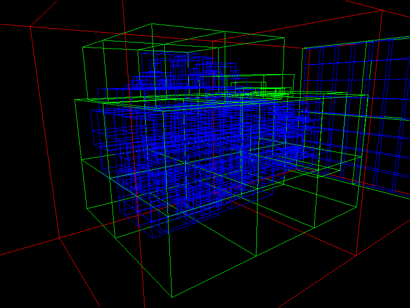
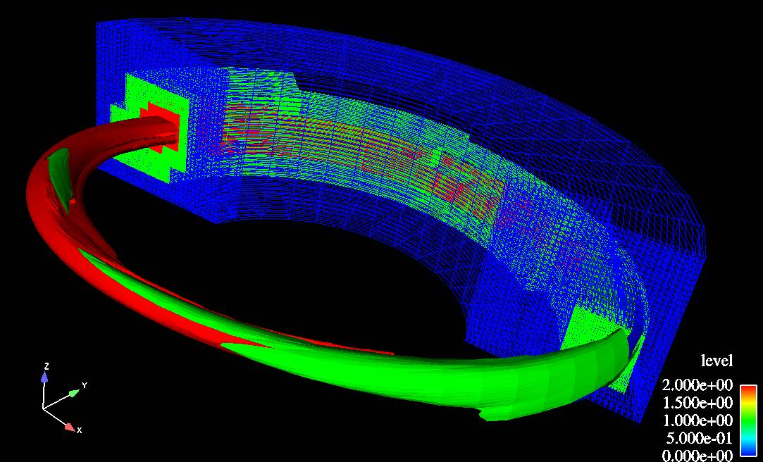
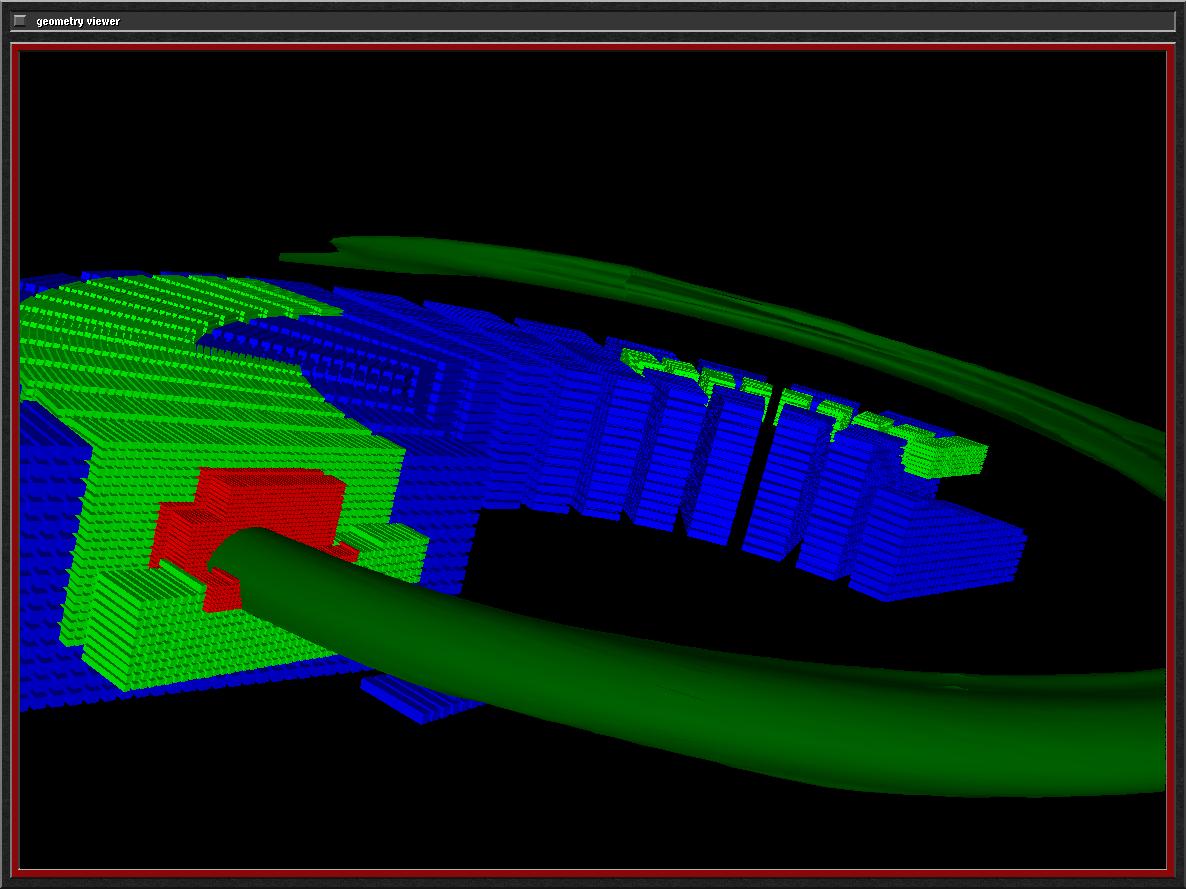
One dataset used in our research is a physics simulation that models the effects of a shock wave passing through an Argon Bubble suspended in air (data courtesy of John Bell and Vince Beckner, LNBL's Center for Computational Sciences and Engineering. The Argon Bubble dataset is defined over a domain of 256 x 256 x 640 cells. Without AMR, a PDE solver would have to compute on 41.9 million grid cells; using AMR, the number is reduced to about 2.9 million (depending on the time step) by building a three-level hierarchy. See Figure 2 for a rendering of this data set and its grid structure. This movie (5.8MB, MPEG-1) shows the first 350 time steps of the simulation, rendered by the single-CPU version of our rendering application.

Figure 2.

Left: The grid structure of an AMR data set. The coarsest-level grids are outlined in red, the finest-level grids are outlined in blue.	Right: A rendering from the same viewpoint, using data from all grid levels.

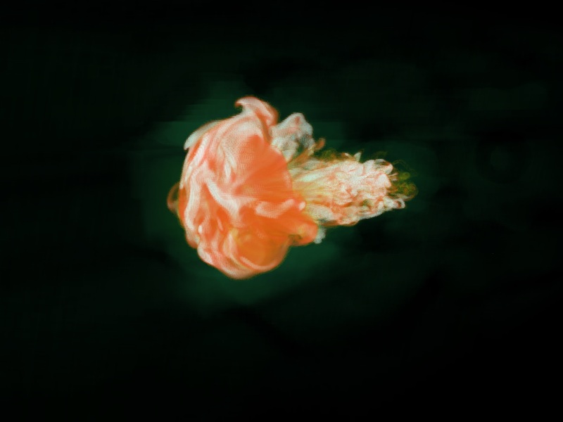
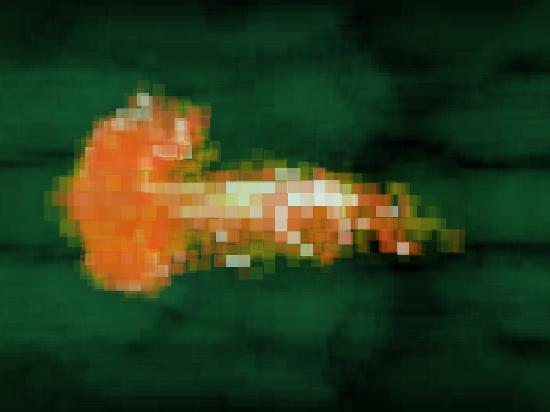
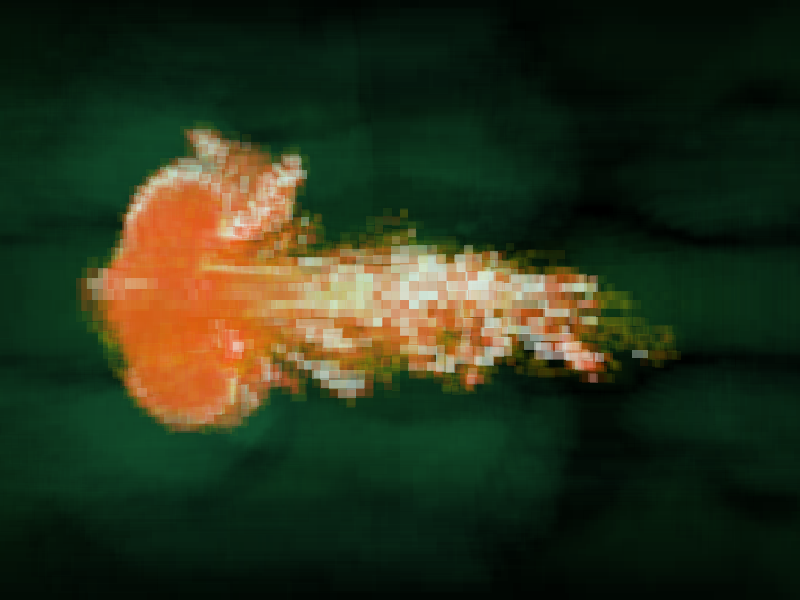
Due to its hierarchical structure, AMR data poses difficult problems for visualization: Most visualization algorithms assume a uniform grid, and in fact, in the past AMR data has been "flattened out," i.e., resampled to the finest resolution grid, in order to visualize it. The additional resampling effort, and the increase in data set size caused by it, made AMR visualization slow and cumbersome. A visualization program that is aware of an AMR data sets inherent multi-resolution structure, on the other hand, can use this to its advantage. For example, the program could allow to render low-resolution preview images by only considering some of the hierarchy levels. Figure 3 shows three different-resolution renderings of the same data set from (approximately) the same view point.


Figure 3: Rendering AMR data sets at multiple levels of resolution.

Getting AMR Data into Existing Visualization Tools

The most computationally and memory efficient way to visualize AMR data is to treat it as a first-class data type and operate directly on its native data structures. Existing off-the-shelf visualization tools and libraries have no concept of native AMR data structures. While new tools like the LBL AMR Volume Renderer, and ChomboVis are taking the first steps towards direct visualization of AMR data structures, it will take many years of development to bring the native AMR visualization algorithms up to the breadth and sophistication of existing tools and frameworks. Some organizations, like PPPL, have come to depend on very sophisticated computational infrastructure built on top of existing tools like AVS/Express, CEI Ensight, and LLNL VisIt.

The visualization group has developed a number of file format convertors that enable scientists to use a variety of turnkey remote/parallel visualizationapplications like the LLNL VisIT, CEI Ensight, VTK, AVS5, and AVS/Express. This provides APDEC customers a broad variety of dataanalysis options for understanding Chombo datasets that complement thecapabilities of ChomboVis. The conversion software converts the grid hierarchy into a hexahedral unstructured mesh. Overlapping cells are removed, and coarse-fine boundaries are stitched in order to minimize rendering artifacts that the boundaries where dangling nodes exist. The tool currently reads the Chomobo HDF5 format and can output data in AVS-UCD, Ensight Gold, and VTK Unstructured file formats (both binary and ASCII form).


Figure 4: The same AMR dataset visualized using VisIt, Ensight, and AVS/Express. The dataset was produced by Ravi Samtaney of PPPL using the Chombo AMR framework. The data is of a pellet of fuel being injected into a Tokamak fusion reactor. The isosurfaces are the density of the pellet material after it has been injected from the interior wall of the reactor.

While the conversion to hexahedral cells has greatly improved the accessiblity of AMR data, it is not an ideal long-term solution. The hexahedral data representation consumes much more memory than the original AMR data and requires algorithms that are more computationally expensive than those that operate on uniform grids. This limits the effectiveness of this method for larger datasets, but still offers an excellent platform for debugging and data inspection before the AMR code scales up to production data sizes.

LBNL Hardware Accelerated Volume Renderer

The goal of this project is to provide a tool that can render AMR data directly, without the intermediate step through a uniform grid or unstructured mesh representation. This tool should run on a wide variety of machine architectures, and should also be accessible through the internet for remote visualization. Currently, the target architectures include:

Single-CPU desktop graphics workstation: On machines of this type (LINUX workstations, windows PCs, etc.) the renderer will use hardware-accelerated rendering methods to achieve interactive frame rates. The current prototype version of this program can render the "Argon Bubble" at an image resolution of 800x600 pixels in about 1.2 seconds on an AMD Athlon 800/GeForce 2 workstation. The same image can be rendered on an SGI Onyx2/IR2 in about 5.6 seconds using a single CPU.
Multi-CPU shared-memory graphics workstation: This renderer uses the same hardware-accelerated rendering methods as the first one; the final compositing step is performed in hardware as well, using image blending. Currently, this program can render the "Argon Bubble" at an image resolution of 800x600 pixels in about 2 seconds on a dual-pipe IR2 SGI Onyx2 using two CPUs. The images of Figure 2 were rendered using this program.
Remote Visualization Server: The renderer can be configured in a client-server configuration where the rendering takes place where the data resides and delivers the results via a network socket to a lightweight client running on the user's workstation. The offscreen rendering is able to use hardware acceleration where available, but can also use the software implementation of the rendering infrastructure. The images computed on the visualization server use variable JPEG compression in order to trade off response time with bandwidth limitations to the client workstation.

Supercomputer

Typical AMR data sets are generated on supercomputers (Cray T3E, IBM SP2), and they are too large to transfer them to smaller machines for rendering. Therefore, the visualization program should also be running directly on the supercomputer generating the data. The goal is to use software rendering in each processing node with final compositing to create the images.

Renderer Architecture

Even though it is aimed for very different machine architectures, the internal structure of the renderer is almost identical for all the versions. Since most rendering algorithms are optimized for uniform grids, the renderer first splits the hierarchical AMR data set into uniform blocks, then renders the blocks independently, and finally composites the partial results. On a single-CPU machine, the rendering and compositing is done sequentially, of course. The overall rendering loop looks like this:

Load data set
Split data set into uniform blocks
Distribute those blocks to the processing nodes
Render each block
Composite the rendering results

Splitting Data Sets

As it turned out, a very simple and efficient method to chop up an AMR data set into uniform blocks is to overlay the data domain with an octree aligned with the finest grid cells in the hierarchy. Then the octree is built recursively by splitting each node that is not completely overlayed by a single grid. The effect of this is that each octree leaf corresponds to a uniform rectilinear grid of data values inside the AMR hierarchy. The result of this octree generation is shown in Figure 4.

Figure 4: Overlaying the data domain with an octree.

Distributing Blocks

We are investigating multiple methods to distribute blocks between processing nodes in the parallel renderer; currently, all of them are based on the octree generated by the splitting stage.

Round-robin Leaf Assignment: The octree leafs generated by the splitting stage are assigned to processing nodes based on their index in an octree traversal. If there are N nodes, then node i will be assigned all the leaves with index N * j + i, where j = 0, 1, 2, ...
Since octree leaves can vary vastly in size, we expect load-balancing problems with this approach. Also, the compositing stage for this distribution method is complicated and involves a lot of communication. On the other hand, the assignment of octree leaves to processing nodes is static and independent of viewing direction, which will reduce I/O overhead during viewpoint animation; furthermore, the increased communication can be overlayed with the rendering itself.
Back-to-front Cell Assignment: Instead of using the octree leaves directly, they are further broken up all the way down to the cell level. Then the resulting octree is traversed in viewing direction, and leaves are numbered on-the-fly, see Figure 5. In a second traversal, each processing node generates a partial image for a stretch of octree leaves: If there are n nodes and N octree leaves in total, then node i will render leaves (N*i)/n to (N*(i+1))/n. This approach is a hybrid between octrees and space-filling curves, in that a linear enumeration of cells is broken up into n pieces of approximately identical cost.
We expect this approach to result in very good load balancing, because the cost of rendering a stretch of cells can be estimated accurately and easily. Also, the compositing step resulting from this distribution is extremely simple, because the partial images can be composited simply in order of processing node numbers. On the other hand, the assignment of cells to processing nodes depends on the viewing direction and might increase I/O overhead during viewpoint animation.

Figure 5:Numbering and assigning cells to processing nodes based on viewing direction, in the case of four processing nodes.

Rendering

In the program versions for graphics workstations, the rendering of octree leaves is hardware-accelerated. In the current program version, a uniform block of data is uploaded to the graphics hardware as a stack of axis-aligned 2D textures which are then rendered into the frame buffer in back-to-front order using the OpenGL compositing operator. In this way, compositing of partial images is performed implicitly during rendering. Due to the limited precision of the frame buffer (typically 8 bits per pixel and color channel) and the amount of texture slices that are composited, the image quality is lower than in the software-only renderer. Switching to 3D textures and view-orthogonal slices will improve image quality only slightly.

The software-only renderer for supercomputers will be based on a cell projection algorithm. First, we will be using a cell projector with piecewise constant interpolation to show off the hierarchical structure of the rendered AMR data sets; later we will incorporate a higher-quality, piecewise linear cell projector based on work done by Nelson Max.

Compositing

The compositing strategy needed to combine the partial images generated on each processing node depends on the distribution strategy used. In the second distribution algorithm (back-to-front cell assignment), compositing is trivial: Due to the nature of distribution, all cells rendered by node i are in front of all cells rendered by all lower-numbered nodes, and are behind all cells rendered by all higher-numbered nodes. Thus, the partial images can be composited in order of node numbers, without having to add a depth channel to the transmitted partial images. To do the actual compositing, we will first implement a simple binary-tree compositing step, and maybe later replace that with the more elaborate binary-swap compositing algorithm.

When assigning octree leaves round-robin, compositing is trickier: Each node renders multiple leaves and has to perform multiple compositing operations, requiring to send multiple partial images between nodes. The additional compositing time, however, can be overlayed with the rendering time: A node will render an image, send it off for compositing, render another (small) image and so on. The index of the node that is responsible for compositing the image generated by an (interior) octree node can be determined by its number; therefore, the compositing does not need to send additional messages on top of the partial images themselves. Each node will be running two processes: One will render octree leaves, the other one will wait for partial images from "child" processing nodes, composite them and send them off towards the octree root. Octree leaves are generally traversed in viewing order, so the previously sequential steps of rendering and compositing can now truly be overlayed.