Wes Bethel
Information and Computing Sciences Division
Lawrence Berkeley Laboratory
The University of California
Berkeley, California 94270
ewbethel@lbl.gov
Janet Jacobsen and Preston Holland
Earth Sciences Division
Lawrence Berkeley Laboratory
The University of California
Berkeley, California 94270
We describe the process used in combining an existing computer simulation with both Virtual Reality (VR) input and output devices, and conventional visualization tools, so as to make the simulation easier to use and the results easier to understand. VR input technology facilitates direct user manipulation of three dimensional simulation parameters. Commercially available visualization tools provide a flexible environment for representing abstract scientific data. VR output technology provides a more flexible and convincing way to view the visualization results than is afforded in contemporary visualization software. The desired goal of this process is a prototype system that minimizes man-machine interface barriers, as well as enhanced control over the simulation itself, so as to maximize the use of scientific judgement and intuition.
In environmental remediation, the goal is to clean up contaminants either by removing them or rendering them non-toxic. A computer model simulates water or chemical flooding to mobilize and extract hydrocarbon contaminants from a volume of saturated soil/rock. Several wells are drilled in the vicinity of the contaminant, water and/or chemicals are injected into some of the wells, and fluid containing the mobilized hydrocarbons is pumped out of the remaining wells. The user is tasked with finding well locations and pumping rates that maximize recovery of the contaminants while minimizing drilling and pumping costs to clean up the site of interest.
In 1965, Ivan Sutherland charted a course for research in computer graphics, which has yet to be fully achieved. He defines the "Ultimate Display" as "a window through which one beholds a virtual world. The challenge to computer graphics is to make the picture look real, sound real and the objects act real." [see 1] Added to this lofty and elusive goal is the notion that we, as human beings, can interact with the objects in this virtual world in a way which is "natural." These two concepts come together to define, in broad terms, computer based "Virtual Reality." Sutherland's vision has guided the computer graphics industry for nearly thirty years.
In contrast, one of the goals of scientific visualization [2] is to "see the unseeable." Rather than pursue the grail of the ultimate renderer and the ultimate motion or deformation model, it is desirable, through abstraction, to make images of what was previously unseeable, or nonexistant. Mathematical formulas, theoretical molecular structures, structures of the galaxies evolving over time, behavior of algorithms, and so forth, are all things that are simply "unseeable." As humans, we tend to believe what we see, and when we see an image of a complex mathematical formula, we tend to believe that the shape that we see is "real." Our acceptance of the images of the "unseeable" is further reinforced when the objects representing the unseeable behave in the same way as objects in the "real" world. They can be picked up, moved around, and so forth. At this juncture, VR and scientific visualization overlap and provide natural complements for one another.
Over the years, the visual and interactive aspects of VR have received much attention. More recently, studies have been undertaken that explore beyond the better-understood visual and interactive aspects of VR. Such studies explore haptic systems that provide tactile feedback ([3], [4]), and the use of sound [5].
We consider the terms Virtual Reality and Virtual Environments to be synonymous, and consisting of three broad components: a computer model which is rendered into an image; the process of user-model interaction; and the process of model viewing.
The model itself is, in broad terms, independent of any VR hardware. A model can come from a variety of sources; a CAD package, visualization tools, imaging tools, and so forth. The model can include, in addition geometric information, dynamic information, such as motion paths or kinematics. In our prototype application, the model consists of visualized simulation output, consisting of geometry and volumetrics, along with simulation parameters represented geometrically. The model, in general, consists of geometric (and possibly volumetric) information. The simulation itself is also a model in it's own right. However, the simulation doesn't appear on the screen as an "object" in the same way as the simulation parameters (the wells, for example). The simulation is manipulated indirectly, while the parameters are directly subject to user control.
Model interaction includes at least two subcomponents. Implementing this man-machine interface requires some type of input device and software which supports updating the model based upon user input. For now, we assume that the final image presented to the user changes whenever the model is changed. We permit the user to directly manipulate a only select set of visualized simulation parameters. Manipulation requires a pick operation, to indicate which of the parameters to edit, and then modifying a location value.
Viewing the model involves three subcomponents. A rendering system is needed which is capable of producing images from a model. Display hardware is used to present the image to the user. Input devices gather user input about viewing parameters. The configuration of hardware and software that we use, along with an overview of design decisions and goals, will be discussed in a later section.
There are numerous software tools that may be used for creating a Virtual Reality (using the definition we have adopted), numerous gadgets that may be used for getting input from the user and for displaying images of this virtual environment. Enumerating these, and providing a taxonomy of devices and the different shades of VR is beyond the scope of this paper. In this paper, discussion of these devices is limited to the actual hardware and software used. See [6] and [1] for more information, such as taxonomies of input and output devices, ranges of VR ranging from Window-on-a-World through complete immersion.
To achieve our goal, namely a VR interface to an existing simulation, we extended a commercially available package for scientific visualization to include VR input, and ported the simulation into this environment. We gain the benefits provided by VR input, namely enhanced control over three dimensional information (the simulation input, and user viewpoint), as well as the benefits of a flexible environment for visualizing scientific data.
We will explore some of the previous work in combining VR with scientific visualization and indicate the relationship between our work and previous studies. A discussion of site remediation, the specific simulation, its parameters, output and how they are visualized and manipulated follows. Finally, number of observations about the process of combining VR technology, a simulation and a dataflow visualization package, and the results of the project are discussed.
Cruz-Neira, et al, describe the CAVE, an immersive environment that employs three-dimensional tracking devices, three-dimensional picking devices, auditory feedback, and a number of projections screens that surround the user, thus forming a "cave" [7]. The CAVE has been used for architectural walkthroughs, cosmic exploration, fractal exploration, viewing the behavior of algorithms implemented on parallel machines, and understanding weather and molecular dynamics [8]. Among the advantages of this type of VR system are the ability to track the user in a confined space providing control over the user environment, a high-resolution stereo display in which each screen has a resolution on the order of 1K by 1K pixels displayed in stereo at 120hz, as well as providing an environment for an immersive experience for a group of participants.
Bryson and Levit have implemented a system called the "Virtual Wind Tunnel" [9]. The purpose of this system is to facilitate the study of flow fields using immersive technology such as the Fake Space BOOM for display and a glove for providing three-dimensional input. A glove is used to specify seed points for releasing particles into the flow field in order to trace their trajectories. The boom-mounted display makes it easy to enter/exit ("unsuit") to/from the virtual environment. Additionally, the BOOM provides the benefit of delivering high-resolution stereo images to the user and has a wide field of view (in contrast to consumer grade head-mounted displays).
Sherman [10] reports VR extensions to two systems for scientific visualization that employ the dataflow paradigm. Dataflow-based packages consist of reusable program modules, which have a consistent interface for inter-module data communication. These systems facilitate experimentation and allow for rapidly bringing new data into the system for viewing and interaction. Dataflow packages are extensible through user-written modules. Sherman's work describes extensions to one such package to support VR input (VPL dataglove) with an input module, and VR output (to the Fake Space BOOM) with a custom rendering module. One premise of this work is that the same environment that is used to create visualization programs can be used to create VR applications for viewing and interacting with scientific data. Hence, users already familiar with the use of one of the dataflow packages will require minimal additional training to use VR.
Our work is most similar to that of Sherman's in the respect that we extend a dataflow package to incorporate VR input and output. Using stereo window-on-a-world VR output (see [1] or [6]), we are able to successfully merge a window into our virtual world with traditional window-system-based GUI's for access to menus, dials and sliders. The combination of control over three dimensional parameters using VR input devices, along with access to scalar parameters via a mouse, allow us to effectively control a simulation for chemical flooding which executes within the dataflow model.
In this section, we discuss the chemical flooding simulation, describing its inputs and outputs, some porting issues, and the extensions we made to a dataflow visualization system.
Site remediation is the process of removing a contaminant from the subsurface. The simulation for this project models water or chemical flooding to remove hydrocarbon contamination. Hydrocarbon contamination can occur as a result of a leaking oil tank or from years of dumping jet fuel on the ground. The parameters that are of primary interest in site remediation are the locations of injection wells into which water or chemicals are injected, in order to mobilize the hydrocarbon, and the locations of production wells from which the fluid containing the hydrocarbon is pumped. The most crucial problems encountered in this type of work are to determine the optimal locations of the injection and production wells together with suitable pumping rates. Optimal placement of wells and pumping rates will result in reduced drilling and remediation costs.
At the start of this project, the simulation itself was in the form of a batch program. The major modifications required to this code involved changing the manner and means by which it obtained input and how it disposed of its output. Such an activity is typical of porting any code into a dataflow package.
The simulation requires as input a three dimensional finite-difference grid, a description of the initial state of subsurface parameters (e.g., permeability, porosity, and initial hydrocarbon distribution and concentration), locations of each of the injection and production wells, the rates of injection and production, and the type of fluid injected (water or a chemical mix).
Given that we wanted to provide visualization tools for not only the input parameters (e.g., the grid, the values of the subsurface parameters at each grid node, etc.), but also allow some of these parameters to be edited by the user (the wells) as wells as display simulation output, the following breakdown of tasks was identified.
A custom module was written which parses the "grid file." The grid file contains information about the spatial structure of the three dimensional finite-difference grid, as well as values of permeability and porosity at each node. The grid-reading module produces as output a structure which can then be visualized in a number of ways. The simplest manner of visualizing the grid is as a wireframe mesh, which simply shows the spatial structure of the grid.
 |
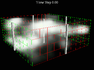
Figure 1 shows a visualization of a three dimensional finite-difference grid, along with an initial placement of wells. In addition, the initial permeability distribution in the grid is visualized using direct volume rendering [11]. Areas of high permeability are more opaque, while areas of lower permeability are more transparent. It is possible to permit the line segments forming the visualized grid to be color-coded according to the values of one or more of the parameters, but in practice, this tends to not work out well (it is hard to interpret), especially when other data is visualized simultaneously with the grid, such as output from the simulation. As an alternate way of visualizing the grid, we also output a cell-based model of the grid. The cell-based model is composed of a number of hexahedral shaped cells, with the permeability and porosity values associated with cell nodes. The user is free to use either of these structures, and a variety of visualization tools, to represent the grid visually as they see fit.
A second module was written which parses the "wells file." This file contains information about the locations of the wells with respect to the grid, the well type (production or injection), injection or production rates, as well as other well parameters. For each well read in, a geometric representation of the well is constructed and passed on as output (to the rendering module of the system). Using feedback loops within the dataflow package, it is possible to detect when the user has performed a pick operation on a particular well. The pick information is typically generated by the rendering module, and is performed using the mouse. When a well pick is detected, that well is highlighted using a color information. Information about that well, such as it's location in the finite-difference grid, is displayed. The user may then make use of the Spaceball to move the well around in the grid (the wells module contains code which reads information from the spaceball device). After completing the editing operation on one well, the user may elect to move another well around, or to run the simulation using new well parameters. In addition to creating the output geometry used to visualize the well locations, this module also creates a text file describing the wells, and associated parameters, for the simulation.
The third component is the simulation module. The process of porting the simulation code into the dataflow environment presents several software engineering challenges, not the least of which is segregating input/output tasks from the rest of the code into structured interfaces. Due to time constraints, and a high level of interdependencies within the code, we elected to leave the simulation input/output facilities in a fairly unmodified form. This means that the simulation still gets its input from text files.
In terms of "porting" the output of the simulation into a form suitable for use in the dataflow environment, the simulation module will accept as input the grid structure produced by the grid module, "throw away" the permeability and porosity values associated with each grid node, and "fill in" values on the grid with chemical concentrations as the simulation proceeds through time. Thus, the user has two grids to visualize. The first, as described in above, contains the structural information about the grid, as well as initial parameters about the subsurface. These parameters are static for the duration of the simulation. The second, computed by the simulation module, contains new values for oil, water, and other chemicals, at each time step at each grid location. Thus, the two grids are identical topologically, but contain different types of information at each node.
The simulation module executes asychronously (once it has all its input parameters specified) from the rest of the dataflow network. As each time step is finished, a new chemical concentration grid is passed as output to the downstream modules in the dataflow network. At the present time, the simulation executes on the same CPU as the dataflow package and the rendering system, which is a graphics workstation. Future plans include porting the simulation to a massively parallel machine, while leaving the visualization and dataflow scheduling tasks to the graphics workstation.
The user is free to experiment with alternate methods of visualizing the grids.
Figures 2 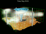 and 3
and 3 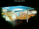 show, from two time steps in the
simulation, the grid, the wells used in this particular run of the
simulation, along with two isosurfaces. The lighter colored isosurface
represents a surface of constant water (injectant) concentration, and
the darker isosurface represents a surface of constant hydrocarbon
concentration.
Figures 4 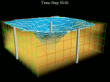 and 5
and 5 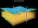 show the use of volume rendering [11],
combined with isoconcentration surfaces, for the same time
steps as figures 2 and 3. Hydrocarbon concentration
is represented with opacity: in areas of high concentration, the
volume appears more opaque, in areas of low concentration, the
volume appears more transparent. These static images are difficult
to interpret, but when the objects in the image are rotated by
the user, the physical structures represented by the volume
rendering become easier to understand.
In summary, porting the "simulation" into the dataflow environment required three custom modules. One is the simulation itself, which computes chemical concentrations on a grid at each time step. A "grid" module reads the grid information, and creates two structures. The user is free to experiment with different visualization techniques to depict either the simulation input grid, along with associated static parameters, or the simulation output grid. The freedom to choose and experiment is a benefit of using the dataflow environment. A "wells" module is the interface to the well editing operation.
At the onset of this work, we were faced with a number of interesting problems. First, UTCHEM, the simulation code used for this project [13], can be characterized as "dusty-deck Fortran", which was developed over time by a number of discipline-science researchers and which was built to be run on a vector machine. Interactivity was not a part of the design of this code, nor was graphical output. Porting this code into a dataflow visualization system required special attention to compatibility issues with regard to simulation input and output. The simulation was written to perform all input and output operations to text files. The dataflow packages make use of data structures or data models for data communication between modules.
Second, at LBL, we make use of dataflow based visualization systems for most visualizations of data. Given their flexibility and extensibility, as well as allowing for modules to execute on remote systems, these environments for visualization and computing make efficient use of existing resources. We wished to leverage upon this efficiency by extending these systems to not only include simulations, but to also act as a testbed or "breadboard" for including VR operations.
Third, we wanted to explore the use of VR as applied to scientific research and the visualization cycle.
Fourth, we wanted to integrate all of these items into one environment that would support making a relatively seamless transition from "desktop" VR (in as much as VR can be done on the desktop) to VR "in the graphics lab." When the first of the dataflow-based visualization systems appeared, they were built to run on a single machine, typically a high-powered graphics workstation. The scientist had to be physically at the console of the workstation to run the system. Aside from being an inconvenience at a large research facility, there was the constant problem of competition for access to the workstation. As the visualization systems evolved to use network-based window systems (e.g., the X windowing system), scientists were then able to do visualization on the desktop. This was immensely popular; the problems of competition and having to be physically in front of the graphics workstation disappeared. The tradeoff, obviously, is one of performance, but the degraded performance was, by and large, acceptable most of the time and viewed as the cost of convenience.
In our graphics laboratory, we are using a DEC Alpha 3000/400, with a Kubota Pacific Denali 6/20 (the graphics engine), a Tektronix stereo shutter, cardboard polarizing stereo glasses, and a Spaceball Technologies, Inc. spaceball. The desktop system is a Sun Sparc 2 with a GX graphics adapter, and a spaceball. We use AVS as the dataflow visualization system. A single module was written for acquiring spaceball events and injecting them into the dataflow network, where they were further processed by modules that place the wells and specify a camera position for the rendering module.
This has been an experiment in which we wanted to maximize the use of very valuable resources, namely scientific knowledge and human intuition. In the virtual environment, the scientist may experiment with simulation parameters and get immediate feedback as to their effect on the simulation. The VR extensions provide a means to easily control three dimensional parameters, something which has been missing in computer simulations.
A set of reusable software tools, combined with commercially available VR gear, commercially available computing equipment and visualization software has been integrated into an environment for experimenting with parameters for a simulation of water/chemical flooding, resulting in enhanced scientific productivity and new insights into a physical system.
The authors would like to thank Akhil Datta Gupta, one of the developers of UTCHEM, for providing valuable assistance in porting the software, as well as for verifying the results and offering useful suggestions for improvements in the prototype system. The authors would also like to thank Harvard Holmes for numerous helpful suggestions which has made this paper more understandable.
This work was supported by the U.S. Department of Energy under Contract No. DE-AC03-76SF00098.
2. McCormick, B., DeFanti, T., and Brown, M. (editors), "Visualization in Scientific Computing (ViSC): Definition, Domain and Recommendations", Computer Graphics, Volume 21, Number 6, 1987.
3. Iwata, H., and Noma, H., "Volume Haptization", Proceedings of the IEEE 1993 Symposium on Research Frontiers in Virtual Reality, pp 16-23.
4. Rosenberg, L, and Adelstein, B., "Perceptual Decomposition of Virtual Haptic Surfaces," Proceedings of the IEEE 1993 Symposium on Research Frontiers in Virtual Reality, pp 46-53.
5. Astheimer, P., "What you See is What you Hear - Acoustics Applied in Virtual Worlds," Proceedings of the IEEE 1993 Symposium on Research Frontiers in Virtual Reality, pp 100-108.
6. Isdale, J., "What is Virtual Reality? A Homebrew Introduction and Information Resource List," Version 2.1, October 1993. Available via ftp from ftp.u.washington.edu.
7. Cruz-Neira, C., Sandin, J., DeFanti, T., "Surround-Screen Projection-Based Virutal Reality: The Design and Implementation of the CAVE," Computer Graphics, Proceedings of Siggraph 1993, pp 135-142.
8. Cruz-Neira, C., Leigh, J., Papka, M., Barnes, C., Cohen, S., Das, S., Engelmann, R., Hudson, R., Roy, T., Siegel, L., Vasilakis, C., DeFanti, T., Sandin, D., "Scientists in Wonderland: A Report on Visualization Applications in the CAVE Virtual Reality Environment," Proceedings of IEEE 1993 Symposium on Research Frontiers in Virtual Reality, pp 59-66.
9. Bryson, S. and Levit, C., The Virtual Windtunnel: An Environment for the Exploration of Three-Dimensional Unsteady Flows, Proceedings of IEEE Visualization 91, pp17-24.
10. Sherman, W., Integrating Virtual Environments into the Dataflow Paradigm, Fourth Eurographics Workshop in ViSC, Workshop Papers, April 1993.
11. Volume Rendering, R. Drebin, L. Carpenter, P. Hanrahan, Computer Graphics, Volume 22, Number 4, Proceedings of Siggraph 1988.
12. Upson, C., et. al., "The Application Visualization System: A Computational Environment for Scientific Visualization," IEEE Computer Graphics and Applications, Volume 9, Number 4, July 1989.
13. Datta Gupta, A., Pope, G. A., Sephernoori, K. and Thrasher, R. L., A symmetric positive definite formulation of a three-dimensional micellar/polymer simulator, SPE Reser. Eng., pp. 622-632, November 1986.