A simple ParaView example will be presented
in this section in order to familiarize you with the basic operation of
the application. More detailed information can be obtained by using the
hyperlinks in this section. A separate tutorial contains several detailed
examples which should be attempted after you are comfortable with the
basics.
Step 1: Start ParaView
If you have installed
ParaView on Windows, you can start the application by using the Start
menu. Under the Programs submenu you will find a ParaView06 menu which
contains ParaView and Check for updates. Select the ParaView item and
you will see the ParaView splash screen. After a few seconds, the application
should appear.
If you have installed
ParaView on Linux or Unix you will need to go to the directory in which
the application is installed, and type ./ParaView.
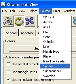
Step 2: Create a sphere
ParaView
starts with an empty scene. At this point you can either load data or
create a source. In this example, we will create a sphere source using
the Source menu in the Menu Bar as shown on the right. Once you select
the Sphere item, the Left Panel will change to display the Selection Window
on top and the Property Sheet for the sphere source on the bottom. The
Accept button on this property sheet will be highlighted in red, indicating
that the data object created by this source is out-of-date. In this case
it has not yet been created. Press the accept button to create the sphere.
You will see a white sphere appear in the Display
For users who are familiar
with VTK, here are the details of what has happened. A vtkSphereSource
was created, and the parameters of this object are presented to you in
the property sheet. When you first create the vtkSphereSource it has an
empty output, and therefore you need to press the Accept button to cause
an Update() call on the sphere source. This is also true when you change
a parameter on the property sheet since the output will then be out-of-date
with respect to the currently displayed parameters.
When you add data to
ParaView (by loading, creating a source, or filtering) a set of objects
are created to manage the data generation, data storage, and display.
ParaView groups these objects together under the name presented in the
property sheet - in this simple example it is Sphere1. When you select
Sphere1 from the Select menu or by using the Selection / Navigation Window,
the property sheet that is displayed contains parameters for the source
object that creates the data, information about the data object that is
created, and controls for the display of the data object. For example,
the Parameters tab contains entry boxes for the center and radius of the
sphere which are variables in the vtkSphereSource. The Information tab
tells you that the data object created by the sphere source contains polygonal
data with 96 cells and 50 points. The Display tab provides controls for
the mapper, actor, and property objects associated with the display of
this data, allowing you to change position, orientation, color modes and
other display attributes.
Step 3: Change to wireframe
The image you see in
the Display Area should be similar to the one shown below on the left.
We will now change the sphere from a solid representation to a wireframe
representation to more easily see the underlying polygons. To do this,
press the Display tab on the property sheet for the sphere shown in the
Left Panel. In the Display Style area, change the Representation from
Surface to Wireframe. The image should now appear similar to the one shown
below on the right.
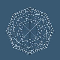
Step 4: Change the resolution
We will
now change the resolution of the sphere. Go to the Parameters tab on the
property sheet shown in the Left Panel. There are two resolution parameters,
Theta Resolution and Phi Resolution, both of which have a default value
of 8. You can see from the silhouette of the spheres shown above that
there are eight segments defining the sphere. Change both of these resolution
values to 12. You will see that the Accept button changes to red indicating
that the displayed object is out-of-date with respect to the parameters
in the user interface. Press the Accept button to see the result of this
resolution change. You should see a sphere similar to the one shown on
the right. This sphere contains more polygons that the previous one and
provides a closer approximation to an actual sphere.
Note that changing the
values and pressing the Accept button did not generate a new data object,
it simply replaced the existing one. If you have changed some parameters
and the Accept button is highlighted in red, but you decide that you would
like to cancel this change, simply press the Reset button. This will restore
the values previously used to generate the data (or the default values
if the data has not yet been generated).
Step 5: Interact with
the sphere
Using
various mouse and keyboard combinations you can control the objects and
the camera in the Display Area. The mouse bindings can be viewed and changed
by selecting the 3D View Properties option from the View menu, then clicking
on the Camera tab. You will see that there are two "styles"
of mouse bindings: one for 2D movements and one for 3D movements. By default
the camera is in 3D movement mode, and the lower area on this property
sheet shows the current bindings. The default bindings are shown in the
image on the right. The top row indicates what will happen when you press
each of the mouse buttons in the Display Area while moving the mouse.
The second row shows the motion that will occur when you press shift plus
the specified mouse button, and the third row shows what will happen when
pressing control plus the specified mouse button. By using the pulldown
menus you can customize this interaction.
For this example, try
using the left mouse button to rotate the scene. Moving the mouse in the
Display Area while holding down the left mouse button will cause the camera
to rotate around the scene. The point about which the camera rotates is
known as the center of rotation. The middle mouse button can be used to
pan (translate) the scene, and the right mouse button can be used to zoom
in and out. These three operations are the most common.
Step 6: Add a bounding
box
In this
step we are going to add a filter to the pipeline. Select the Outline
item from the Filters menu on the Menu Bar. After you do this you will
see the Outline property sheet appear in the Left Panel. As with sources,
you need to click the Accept button to actually add this filter to the
pipeline. Once you do this you will see an outline box surrounding the
sphere. You will also notice that in there are now two items listed in
the Selection Window: Sphere1 and Outline0. Both items are visible so
an open eye is shown to the left of each. The Outline0 object is the active
data object (if another filter is added it will be connected to this data
object) and is highlighted in yellow.
Use the Display tab
for Outline0 to change the color of the line by clicking on the Actor
Color button in the Color region. You can also change the thickness of
the line using the Line Width slider that can be accessed by clicking
on the small triangle to the right of the text entry box, or by typing
a number directly in the box.
To access the properties
of the Sphere1 you can either click on Sphere2 in the Selection Window,
or select this item from the Select menu on the Menu Bar. This will cause
Sphere1 to be the currently active object, and the Sphere1 property sheet
will be displayed. Using the Display tab change the sphere back to a surface
representation. The image you have now should appear something like the
one shown above.
Step 7: Shrink the sphere
We will now apply another
filter to the sphere. First, make sure that Sphere1 is the highlighted
item in the Selection Window so that the filter we add will be connected
to it. Now select the Shrink filter from the Filter menu. On the property
sheet, change the Shrink Factor to 0.75 (the default is 0.5) and press
Accept. You will notice that several things happen. First, a new item
is added to the selection window called Shrink0 and it is now the currently
selected item. In the Display Area it appears that the polygons defining
the sphere have each been shrunk to 75% of their original size. Actually,
the original sphere (with full size polygons) is still there, it is just
not visible now. Note that the eye icon next to Sphere1 in the Selection
Window is now light grey indicating that this item is invisible. When
the shrink filter was added, and new data object was created based on
the input data object (the sphere). This new object (the output of the
shrink filter) is now visible and the original input is not visible.
Most filters do turn
off the visibility of the input data object when they execute. Two exceptions
to this are the outline filters (Outline and Outline Corners) since it
is assumed with these filters that the user wants to see both the original
data and the filter output simultaneously.
In this example you
have created a branching pipeline in ParaView. You can see this in the
Navigation Window. To change from Selection Window to Navigation Window,
click on the icon next to the Selection Window title.
You should see the title change to Navigation Window, and in the window
you should see:
The item shown in dark
grey is the currently selected data object. All other items are shown
in blue indicating that you can click on that data object to select it.
Click on the Sphere1 item and the display in the Navigation Window should
change to this:
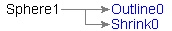
This is a simple representation
of the underlying VTK pipeline. We have create a vtkSphereSource that
has output vtkPolyData which is used as input to both the vtkOutlineFilter
and the vtkShrinkFilter.
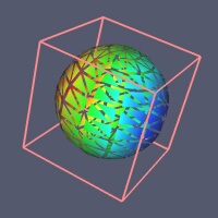
Step 8: Color by normals
Select
the Shrink0 item from the Selection / Navigation Window to access the
property sheet for this item. On the Display tab, change the Color By
option in the Color region to Point Normals 1. You should now see an image
similar to the one shown on the right. Instead of using a specified solid
color for the color of the object, the color is derived from a lookup
table based on some property of the data. In this case we have chosen
to use the Y value of the Normal to look up a color between blue and red.
You can change the current
color map using the Edit Color Map button in the View region. This will
change the property sheet displayed in the Left Panel to one that can
be used to control the color map and the various properties of the scalar
bar. In the Color Map region you can change the two endpoint colors of
the color map. An HSV interpolation strategy is employed for intermediate
values.
 ParaView
starts with an empty scene. At this point you can either load data or
create a source. In this example, we will create a sphere source using
the Source menu in the Menu Bar as shown on the right. Once you select
the Sphere item, the Left Panel will change to display the Selection Window
on top and the Property Sheet for the sphere source on the bottom. The
Accept button on this property sheet will be highlighted in red, indicating
that the data object created by this source is out-of-date. In this case
it has not yet been created. Press the accept button to create the sphere.
You will see a white sphere appear in the Display
ParaView
starts with an empty scene. At this point you can either load data or
create a source. In this example, we will create a sphere source using
the Source menu in the Menu Bar as shown on the right. Once you select
the Sphere item, the Left Panel will change to display the Selection Window
on top and the Property Sheet for the sphere source on the bottom. The
Accept button on this property sheet will be highlighted in red, indicating
that the data object created by this source is out-of-date. In this case
it has not yet been created. Press the accept button to create the sphere.
You will see a white sphere appear in the Display 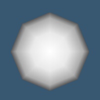
 We will
now change the resolution of the sphere. Go to the Parameters tab on the
property sheet shown in the Left Panel. There are two resolution parameters,
Theta Resolution and Phi Resolution, both of which have a default value
of 8. You can see from the silhouette of the spheres shown above that
there are eight segments defining the sphere. Change both of these resolution
values to 12. You will see that the Accept button changes to red indicating
that the displayed object is out-of-date with respect to the parameters
in the user interface. Press the Accept button to see the result of this
resolution change. You should see a sphere similar to the one shown on
the right. This sphere contains more polygons that the previous one and
provides a closer approximation to an actual sphere.
We will
now change the resolution of the sphere. Go to the Parameters tab on the
property sheet shown in the Left Panel. There are two resolution parameters,
Theta Resolution and Phi Resolution, both of which have a default value
of 8. You can see from the silhouette of the spheres shown above that
there are eight segments defining the sphere. Change both of these resolution
values to 12. You will see that the Accept button changes to red indicating
that the displayed object is out-of-date with respect to the parameters
in the user interface. Press the Accept button to see the result of this
resolution change. You should see a sphere similar to the one shown on
the right. This sphere contains more polygons that the previous one and
provides a closer approximation to an actual sphere.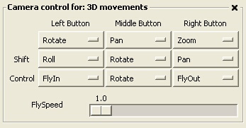 Using
various mouse and keyboard combinations you can control the objects and
the camera in the Display Area. The mouse bindings can be viewed and changed
by selecting the 3D View Properties option from the View menu, then clicking
on the Camera tab. You will see that there are two "styles"
of mouse bindings: one for 2D movements and one for 3D movements. By default
the camera is in 3D movement mode, and the lower area on this property
sheet shows the current bindings. The default bindings are shown in the
image on the right. The top row indicates what will happen when you press
each of the mouse buttons in the Display Area while moving the mouse.
The second row shows the motion that will occur when you press shift plus
the specified mouse button, and the third row shows what will happen when
pressing control plus the specified mouse button. By using the pulldown
menus you can customize this interaction.
Using
various mouse and keyboard combinations you can control the objects and
the camera in the Display Area. The mouse bindings can be viewed and changed
by selecting the 3D View Properties option from the View menu, then clicking
on the Camera tab. You will see that there are two "styles"
of mouse bindings: one for 2D movements and one for 3D movements. By default
the camera is in 3D movement mode, and the lower area on this property
sheet shows the current bindings. The default bindings are shown in the
image on the right. The top row indicates what will happen when you press
each of the mouse buttons in the Display Area while moving the mouse.
The second row shows the motion that will occur when you press shift plus
the specified mouse button, and the third row shows what will happen when
pressing control plus the specified mouse button. By using the pulldown
menus you can customize this interaction.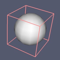 In this
step we are going to add a filter to the pipeline. Select the Outline
item from the Filters menu on the Menu Bar. After you do this you will
see the Outline property sheet appear in the Left Panel. As with sources,
you need to click the Accept button to actually add this filter to the
pipeline. Once you do this you will see an outline box surrounding the
sphere. You will also notice that in there are now two items listed in
the Selection Window: Sphere1 and Outline0. Both items are visible so
an open eye is shown to the left of each. The Outline0 object is the active
data object (if another filter is added it will be connected to this data
object) and is highlighted in yellow.
In this
step we are going to add a filter to the pipeline. Select the Outline
item from the Filters menu on the Menu Bar. After you do this you will
see the Outline property sheet appear in the Left Panel. As with sources,
you need to click the Accept button to actually add this filter to the
pipeline. Once you do this you will see an outline box surrounding the
sphere. You will also notice that in there are now two items listed in
the Selection Window: Sphere1 and Outline0. Both items are visible so
an open eye is shown to the left of each. The Outline0 object is the active
data object (if another filter is added it will be connected to this data
object) and is highlighted in yellow. icon next to the Selection Window title.
You should see the title change to Navigation Window, and in the window
you should see:
icon next to the Selection Window title.
You should see the title change to Navigation Window, and in the window
you should see: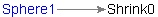
 Select
the Shrink0 item from the Selection / Navigation Window to access the
property sheet for this item. On the Display tab, change the Color By
option in the Color region to Point Normals 1. You should now see an image
similar to the one shown on the right. Instead of using a specified solid
color for the color of the object, the color is derived from a lookup
table based on some property of the data. In this case we have chosen
to use the Y value of the Normal to look up a color between blue and red.
Select
the Shrink0 item from the Selection / Navigation Window to access the
property sheet for this item. On the Display tab, change the Color By
option in the Color region to Point Normals 1. You should now see an image
similar to the one shown on the right. Instead of using a specified solid
color for the color of the object, the color is derived from a lookup
table based on some property of the data. In this case we have chosen
to use the Y value of the Normal to look up a color between blue and red.