This is an archival copy of the Visualization Group's web page 1998 to 2017. For current information, please vist our group's new web page.
Automatic Beam Path Analysis of Laser Wakefield Particle Acceleration Data
Motivation:
Laser wakefield particle accelerators (LWFAs) can accelerate particles to high energy levels over very short distances. LWFAs utilize an electron plasma wave to accelerate charged particles (e.g., electrons) to high energy levels and can create and sustain electric and magnetic fields several thousand times stronger than possible using conventional technologies. Researchers at the LOASIS program have demonstrated high-quality electron beams at 0.1 to 1 GeV using mm long plasmas [2, 3].
Analysis,
understanding, and control of the complex physical processes of
plasma-based particle acceleration is a challenging task and requires
one to understand how particles become trapped in the plasma wave and
how particle beams are formed and accelerated. These processes are best
understood by tracing the particles that form a beam over time and
investigating their temporal evolution. In real-world experiments it
is, however, impossible to record the complete evolution of an
experiment and much less to trace single particles within a
plasma.Numerical
simulations of laser wakefield particle accelerators, hence, play a key
role
in the understanding of the fundamental physics of
plasma-based acceleration, understanding of the processes observed in
experiments, as well as improvement of experiments.
As the size and complexity of simulation output grows, one main challenge is the need for computational techniques that aid in scientific knowledge discovery. One main feature researchers are interested in are beams of high-energy particles formed during the coarse of LWFA simulations. To enable efficient and accurate analysis of these particle beams, dedicated mechanisms for selection and detection of particle beams are needed.
Overview:
The
automatic beam path analysis consists of a set of data-understanding
algorithms that work in concert in a pipeline fashion to
automatically locate and analyze high energy particle bunches
undergoing acceleration in very large simulation datasets [1].
These
techniques work cooperatively by first identifying features of
interest in individual time steps, then integrating features across
time steps, and based on the information derived perform analysis of
temporally dynamic features. This combination of techniques supports
accurate detection of particle beams enabling a deeper level of
scientific understanding of physical phenomena than has been possible
before. By combining efficient data analysis algorithms and
state-of-the-art data management based on H5Part and FastBit we
enable high-performance analysis of extremely large particle datasets
in 3D. The automatic analysis of particle beams based on temporal
particle paths enables accurate classification of particle beams and
supports analysis of the temporal beam evolution.
Algorithm Design:
 |
||
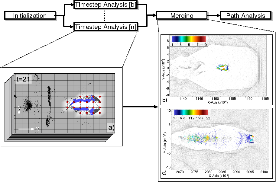
| Figure
1:
After initalization and identification of the relevant time steps, the
different timestep are first analyzed independently to detect the most
prominent particle bunch at each timestep using a combination of
efficient grid-based analysis methods (a).
The results are merged to define a single consolidated description of
each bunch based on the information from the different time steps (b-c). In the example dataset the
algorithm detected two separate bunches shown in figure b and c.
Based on this information the algorithm identifies for each bunch a set
of reference particles that belong with high propabilty to the bunch
(red particles). |
 |
||
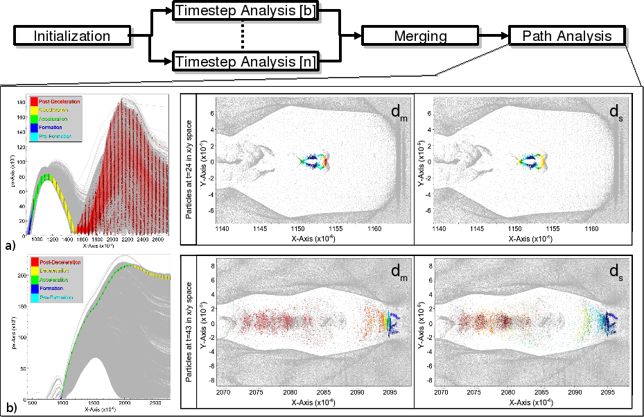
| Figure
2:
In the final path analysis step the algorithm first computes a single
reference path for each bunch bases on the temporal paths of the
reference particles (colored paths in the bottom left images). Based
the reference path the analysis derives the different temporal phases
of a bunch, e.g., when was a bunch formed (blue) or accelerated (green)
(see left figures). Finally, the algorithm computes for each candidate
particle the distance of its path in physical space (ds) and
momentum space (dm)
to the reference path. Based on these bunch distance fields the user
can effectively and intuetively define the bunches. Figure a, b provide an overview of the path
analysis for the two bunches detected in the example dataset. Left: Paths of all candidate
particles (gray) and the reference particles colored according to the
temporal phases of the bunch. Right:
Overview of the path distance fields dm and ds for
the two detected bunches. |
Performance:
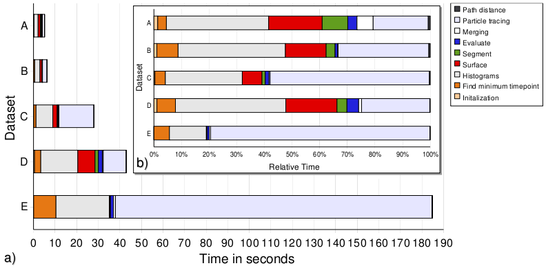
For the example 2D datasets our implementation was able to complete the analysis in less than 45 seconds in all cases. Even in the case of the large 3D dataset —which was produced by a hundred-thousand-processor-hour class simulation— the analysis took only ~185 seconds.
 |
||
| Figure
3: a) Absolute timings
for the serial analysis of five different datasets using the automatic
beam path analysis method. The length of each horizontal bar represents
the total time used for the complete analysis of the corresponding
dataset. b) Relative timings
for the different steps of the analysis pipeline as percentage of the
total analysis time. In both figures color is used to indicate the
timings of different parts of the algorithm. In all cases the histogram
computation and the particle tracing are the most expensive analysis
steps. This is expected since these are the two main steps during which
the raw data needs to be accessed. We can see that the algorithm shows
good performance in all cases and scales well with increasing dataset
size |
Results:
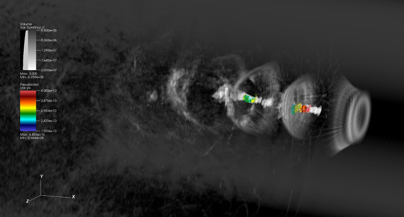 |
||
| Figure 4: Example illustrating the application of the automatic beam path analysis to a large 3D particle dataset (E). The particles of the two detected particle bunches are shown in color with color indicating momentum in x direction (px). A volume rendering of the plasma density (gray) illustrates the plasma wave. |
References
[2] C.G.R. Geddes, C. Toth, J. van Tilborg, E. Esarey, C. Schroeder, D. Bruhwiler, C. Nieter, J. Cary, and W. Leemans, “High-Quality Electron Beams from a Laser Wakefield Accelerator Using Plasma-Channel Guiding,” Nature, vol. 438, pp. 538–541, 2004, LBNL-55732.
[3] W. P. Leemans, B. Nagler, A. J. Gonsalves, C. Toth, K. Nakamura, C. G. R. Geddes, E. Esarey, C. B. Schroeder, and S. M. Hooker, “GeV electron beams from a centimeter-scale accelerator,” Nature Physics, vol. 2, pp. 696 – 699, 2006