This is an archival copy of the Visualization Group's web page 1998 to 2017. For current information, please vist our group's new web page.
Dec 05, 2003
After much thrashing, we have finally jumped through all the hoops necessary to release the Visapult source code. Follow the "Download the Visapult2 Source" link in the Table of Contents (below). Sorry for the delay, and thanks for your patience.
Visapult 2.0
Table of Contents
- Introduction
- Differences from Version 1
- Download the Visapult2 Source (Modified 5 Dec 2003)
- Additional 3rd Party Software You'll Need
- Compiling Instructions
- Execution Instructions
- Viewer Command Line Arguments
- Data Formats Supported by the backEnd
- Future Plans
- Older Visapult project pages.
Introduction
Visapult is an application and framework used for remote and distributed, high performance direct volume rendering. The Visapult application consists of two software components that work together in a pipelined fashion in order to perform volume rendering. The two software components consist of a viewer, which runs on your desktop machine, and which presents a GUI along with support for interactive transformations of the volume rendering. The other component, called the backEnd, runs on some other machine, and performs that tasks of data loading and partial rendering. The viewer, running on the desktop, is able to achieve interactive frame rates even with extremely large datasets due to its use of Image Based Rendering Accelerated Volume Rendering. The viewer requires OpenGL support on the display workstation, along with OpenRM Scene Graph, an Open Source scene graph distribution (see the Download and Compile sections for more details).
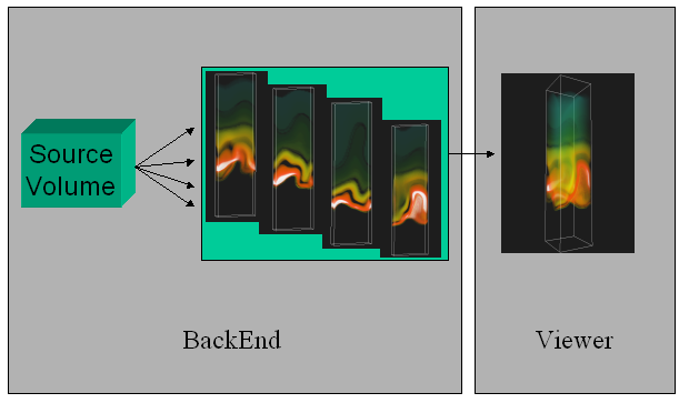
Each of the backEnd and viewer are parallel programs. The backEnd is a distributed memory application that uses MPI as the parallel programming and execution framework. As such, the backEnd will run on any platform that supports MPI programs. The backEnd will read the raw scientific data using domain decomposition strategy that seeks to equally balance the amount of data to be read and processed by each PE. Each backEnd PE reads data and renders, using a software compositing algorithm, in parallel. The results of this activity are then sent to the viewer. For each backEnd PE, there exists a separate TCP communication channel to a corresponding execution thread within the viewer. Unlike the backEnd, the viewer is parallelized using pthreads, and is intended to be run on a single workstation. The viewer can benefit from multiple CPUs on any SMP platform, so best performance will occur when the viewer is run on an SMP platform, such as a multi-processor SGI, Sun or x86.
Differences from Version 1
Visapult was first created as part of DOE's Next Generation Internet program, during the period of 1999-2000. In its first incarnation, the Visapult backEnd domain-decomposed data into slabs. Each slab consisted of an approximately equal number of slices of raw volume data. The width and height of each slab corresponded to the width and height of the volume data, and the number of slices of data, or the depth of each slab, was a function of the number of backEnd PEs and the size of the original volume. The slab-decomposition worked well for it's intended use - high performance volume rendering - but showed limitations in terms of load balancing as well as in terms of usefulness as a visualization tool.
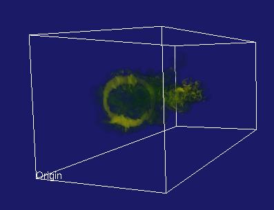
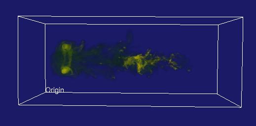
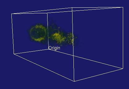
The primary difference between Visapult 1.0 and Visapult 2.0 is that the backEnd and viewer now use a block decomposition strategy, rather than a slab decomposition. A block decomposition lends itself better to even load balancing amongst backEnd PEs. In addition, the backEnd will now render each block from each of the six primary coordinate system axes, and transmit 6x images per block to the viewer. Inside the viewer, as the model is interactively transformed, one of these six images per block is displayed, depending upon the orientation of the model and the viewer. We call this capability "omniview", and its introduction produces better usefulness in terms of visualization.
| Visapult without Omniview | ||
|---|---|---|
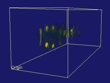
|
|
|
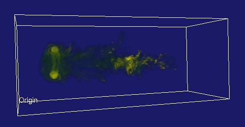
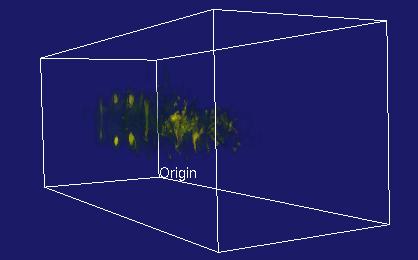
Visapult With Omniview |
|
|
|
Whereas Visapult 1.0 was designed to show that a single application can make effective use of network resources, Visapult 2.0 is oriented more towards providing better visualization services. The omniview capabilities incur a sixfold increase in rendering cost in the backEnd, when compared to Visapult 1.0. This behavior can be disabled when maximum performance is desired, but a recompile is required.
Download
03 Jan 2006 The Visapult-2 source tarball has been moved to LBL's Codeforge Server.
- The significant
change in this version is that you must now specify the network parameters
used by the backEnd and viewer. Two command line arguments are required
for the backEnd: -viewer hostname.domain.com specifies the name of
the host where the viewer is running, and -port portNum specifies the
port number used for the backEnd-viewer connection. See below in the
sections on viewer and backEnd command line arguments for more
details.
- Linux x86 viewer : Precompiled statically linked visapult-2 viewer for Linux x86 systems
- Irix 6.5.x -n32 viewer : Precompiled statically linked visapult-2 viewer for SGI Irix systems
- 11/26/2002 This tarball contains src for the Visapult version used to win the SC02 Bandwidth Challenge. The incremental difference from previous versions is new code that implements a "Cactus UDP" reader. For more information about the Cactus UDP reader, see below in the Cactus UDP data formats section of the document. As a forewarning, the backEnd component is configured in this distribution to not use detached reader and sender threads. If maximum perforamnce is required, you'll need to modify backEnd/main.cxx, searching for "detachedReader" and "detachedSender", changing the initial values for these two variables from zero to one.
- 11/10/02 This tarball contains a fix for an occasional viewer lockup. The lockup was caused by some stale socket manipulation code used to set the TCP window size between the viewer and backEnd. The TCP window code has been updated, along with some naming consistency improvements in the socket library used by Visapult. There are no command line argument changes, or other new functionality in this code drop.
- 11/07/02 This tarball contains a bug fix for the DBLOCKS file format. New under-the-hood features include a separate TCP control line between the viewer and backEnd, needed to communicate control info in the presence of asynchronous payload transfers.
- 11/05/02 The backEnd will now run w/o a viewer. The viewer tells the backEnd how many omniview images to generate - the default is 6. Use the -no-omni command line option when launching the viewer to tell the backEnd to generate (render) only a single image (maximum performance, minimum vis capability).
- 10/29/02 A CVS export of the rtag Oct292002. Contains preliminary support for the DBLOCKIO reader.
- 10/14/02 A CVS snapshot taken on 14 Oct 2002. Contains preliminary support for the BLOCKIO reader.
- 10/08/02 This tarball is a snapshot from CVS on 10/2/2002. There will likely be many more tarballs between now and SC02. This tarball includes source for the Visapult viewer and backEnd, along with some sample data files in AVS volume format.
Additional 3rd Party Software You'll Need
Additional Software for the Viewer
- OpenRM Scene Graph v1.5.0
You will also need to grab a copy of OpenRM Scene Graph, which is the rendering engine used by the Visapult viewer. More information about OpenRM is available at the OpenRM website. Specifically, you need to grab a copy of openrm-devel-1.5.0.tgz. Build and install instructions for OpenRM are listed at the OpenRM website. If you install openrm-devel into /usr/local/rm150 on your machine, you won't have to modify any of the default config files for the viewer later on. You are free to install it anywhere you want, but will have to fix up Makefiles if you do.
- The Fast Light Toolkit (FLKT) v1.1.1
Finally, the viewer program also depends upon the Fast Light Toolkit (FLTK) for its GUI. You can download FLTK from the FLTK website. We have built and tested with version 1.1.1 (the viewer should work OK with version 1.1.2, which is the most recent). The viewer Makefiles assume that the FLTK headers are installed under /usr/local/include, and that the FLKT library is installed in /usr/local/lib. For the impatient, you can grab this tarball: fltk-1.1.1-linux.tgz, which has the FLTK 1.1.1 headers and libs built for Linux (RH 7.3). To install, download the tarball to /tmp, then do the following as root:
	cd /usr/local
	gunzip -dc /tmp/fltk-1.1.1-linux.tgz | tar xvf -
Additional Software for the backEnd
- The Message Passing Interface (MPI)
The backEnd uses MPI as the parallel programming framework. Many vendors provide an implementation of MPI with their OSs. On Linux, we use MPICH, which you can download from the ANL website. That distribution contains instructions for compiling and installing MPICH on your workstation or cluster. We assume that you will have an adeqaute MPI or MPICH infrastructure in place.
Compiling Instructions
- Decide where to unpack the distribution.
- When you tar xvfz the distribution, it will expand into a directory structure that looks like this:
	visapult-2/
	visapult-2/backEnd
	visapult-2/common
	visapult-2/viewer
Ideally, you'll have this directory be located on an NFS-mounted filesystem that will be visible to all nodes that will be running the backEnd. You can unpack the distribution onto a second machine where you'll be running the viewer, as well. - When you tar xvfz the distribution, it will expand into a directory structure that looks like this:
- Prepare to compile
- First, you need to run the makelinks.csh script, which will create symlinks from backEnd and viewer into common so that common code will be available in both directories. You need to perform this step on each machine where you'll be compiling. For example, you'll do this step once on the cluster, and once on your desktop machine where you'll be running the viewer. If all code is on a single filesystem that is visible to all platforms (backEnd and viewer), then you have to do this only once.
	cd visapult-2
	./makelinks.csh
- Build the backEnd
- Since we don't use any sort of autoconf facility, you'll probably need to edit some Makefiles. cd into visapult-2/backEnd, and edit Makefile. There are lines that look like this:
# MPI definitions
include mpich.linux
#include mpich.solaris
#include mpi.irix6
Building for IRIX As listed, this will include the file mpich.linux, which contains definitions that are used for building the backEnd on Linux. Our test system was a RH 7.3 dual Athlon 760MPX system using MPICH 1.2.4, which you can download from the ANL website. If you are compling the backEnd for use on a Linux system, no changes are required. Just type "make" from the visapult-2/backEnd directory.
Building for IRIX- If you want to compile the backEnd for an IRIX system, uncomment the line that reads "include mpi.irix6", and comment out the mpich.linux line. The changes to the above Makefile fragment would look like this:
# MPI definitions
#include mpich.linux
#include mpich.solaris
include mpi.irix6
Then type "make" from the visapult-2/backEnd directory.
- The mpi distributions for IRIX vary somewhat, and you may need to modify the mpi.irix6 line. In our experience, on one platform, the -lmpi++ library is required, while it is not even present (and apparently not needed) on other platforms. We tested the Visapult backEnd on an SGI Onyx3400 running very recent version of IRIX (6.5.18?), and on an SGI Onyx2 running a slightly outdated version of IRIX (6.5.15?).
- Build the Viewer
- Make sure that you have installed OpenRM onto the machine where you will be building and running the viewer. We install it into /usr/local/rm143 on our platforms, and the makeinclude files in the visapult-2/viewer directory assume that location. If your final location for OpenRM is different, please update the appropriate makeinclude.[arch] file first. The viewer/Makefile included in the distribution tarball assumes that you are building for Linux.
- cd into visapult-2/viewer, and type "make."
- Since we don't use any sort of autoconf facility, you'll probably need to edit some Makefiles. cd into visapult-2/backEnd, and edit Makefile. There are lines that look like this:
Execution Instructions
Here's the recipe for running the application:
- Launch the viewer application.
- Go to the viewer machine, cd into visapult-2/viewer, set the LD_LIBRARY_PATH variable to point to the location of the OpenRM .so files, and launch the viewer by typing "./viewer". That's it. No config files are needed for the viewer. You must launch the viewer before launching the backEnd. This restriction will be lifted in a later Visapult release.
- Set up the configuration file visapult-2/backEnd/mpiclient-config
- This text file contains the means to tell the backEnd the hostname or IP number of the machine where the viewer will be running. The comments inside that file are reasonably self-explanatory. You will need to change the contents of this file in order for the application to work. As a further note, it will be a bad idea to run the viewer and backEnd such that they are separated by a packet-filter firewall. It is possible to do, but requires setting up port-forwarding on your firewall (see visapult-2/common/visapult.h, and look for VISAPULT_LISTEN_PORT to see which port the viewer uses to listen. The backEnd uses ephemeral ports for outbound connections). There are few command line options for the viewer, most of which are not implemented. Type "viewer -usage" for information. Chances are, you will not need to use any of them.
- Launch the backEnd
- Assuming that you've modified the mpiclient-config file, here's a quick "hello world" command line you can use to quickly test if things are configured correctly:
mpirun -np 1 ./backEnd -data avs ../data/hydrogen.dat -res 4
- This will run the backEnd application on one PE, reading and rending the small AVS file "hydrogen.dat", which is included with the distribution. You should see some diagnostic text being printed as the backEnd executes, and if all's well, you'll see the viewer respond, and will see an image that you can rotate (with the middle mouse button) or translate in the view plane (with the left button).
- Go to the viewer machine, cd into visapult-2/viewer, set the LD_LIBRARY_PATH variable to point to the location of the OpenRM .so files, and launch the viewer by typing "./viewer". That's it. No config files are needed for the viewer. You must launch the viewer before launching the backEnd. This restriction will be lifted in a later Visapult release.
- You can grab a more substantial data file: small-fdpss-x86.tgz (52MB). Unpack this tarball into /tmp on the machine where you will be running the backEnd. If you want to run on a cluster, copy and extract the tarball into /tmp on each machine : you want the backEnd to have access to the same file on each machine, and putting it in /tmp will allow for fast reads from local disk. Beware that this file will inflate to about 492MB in size when uncompressed. The data in this file (inside small-density, in particular), is IEEE floats written from an x86 (big-endian) machine. You will not be able to use this data on an SGI without first performing a manual endian-conversion on the data. Note that "dd conv=swab" will not do the job of endian conversion. However, this small C source program will do endian conversion.
- The small-fdpss-x86.tgz file contains 3 steps' worth of data from a turbulent flow simulation. The grid resolution is 640x256x256. The work was performed by the Center for Computational Sciences and Engineering group at LBNL.
- To run using this more substantial file, unpack into /tmp as
indicated. Start the viewer as instructed above. Then, start the
backEnd as follows:
mpirun -np 4 ./backEnd -data fdpss /tmp/small-config -pal ./sc99Palette -res 4
You can alter the number of PEs, if you so choose to a greater or lesser number. The backEnd will attempt to do self-load balancing by dividing up the number of data points read and processed by each PE so that all have an approximately equal amount of data. - More details will be forthcoming soon...Note that most of the information on the older Visapult pages concerning job launching and command-line arguments are now invalid. The information on this page is the most current.
Viewer command line arguments (Updated 7 Jan 2003)
- Specify whether or not to use the graphical user interface.
[-gui] | [-nogui]
The -gui option enables the graphical user interface (menus, buttons, etc.) and is the default behavior when neither of -gui or -nogui is specified. The -nogui option turns off all GUI capabilities. When using -nogui, press either 'q' key to terminate the viewer. For example:viewer -nogui
will run the viewer without the GUI. On the other hand,viewer -gui
will run the viewer with the GUI. If you don't specify either of -gui or -nogui, you get the GUI.
- Specify the number of Omniview IBR images .
[-no-omni]
By default, the viewer tells the backEnd to generate six omniview images per block. Then, when you rotate the model around, the best set of images is displayed. Rendering all six images takes a bit of extra time, so you can instruct the viewer to tell the backEnd to render only one, rather than six images. Specificing -no-gui will improve backEnd execution performance at the expense of visualization capabilities. For example,viewer -no-omni
will cause the viewer to request only one IBR image from the backEnd, rather than six, which is the default. If you don't specify anything, you get six IBR images.
- Specify the port number (New 7 Jan 2003)
[-port portNum]
You can specify a non-default port number with this command-line option. Any port value in the range 1024 < n <= 65534 will be accepted. The viewer and backEnd create a pair of sockets as part of the run. The first socket, the control line, is created on the port "portNum." Thereafter, each backEnd PE will connect to the viewer to send payload data at "portNum+1". Default values are provided in the viewer and backEnd code, so this argument is optional. Note that if you do use this option, be sure to use the same port number when you run the backEnd, otherwise the viewer and backEnd will never connect with one another.
Visapult backEnd Command Line Arguments (Modified 7 Jan 2003)
This section explains all of the command line arguments to the backEnd part of Visapult.
- Define the Data Source: -data <type> <filename>
This is a required command-line argument.
As of the time of this writing (10/9/02), the backEnd can read two types of data. The first is scalar byte data stored in AVS Volume format. The second is what we call "FDPSS" format. The name FDPSS has historical connotations, and means "file-based distributed parallel storage system." Basically, the FDPSS format consists of a small ASCII config file, and other files that contain raw binary information. To specify a data source to the backEnd, you use the "-data type fname" command line argument. The two examples that follow read in an AVS volume file (one included with this distribution), and the other reads in an fdpss file.
backEnd -data avs ../data/hydrogen.dat
backEnd -data fdpss /tmp/small-config
backEnd -data blocks /tmp/blocks/small-config
backEnd -data cactusudp IP:port
The string following the "-data" indicates the type of data. At this time, that string must be one of "avs","fdpss" or "blocks". Following the type string is a filename of the data source.
- Define the granularity of block decomposition: -res N (N is a positive integer)
This is an optional command-line argument.
The "-res N" command line argument defines how many blocks will be used in the block decomposition of a given data set. N is a non-negative integer, e.g., 2, 4, 8, etc. It need not be an even power of two, but we have seen strange behavior when set to strange values, and this is under investigation.
The way this parameter works is as follows. Assume that you have a 3D volume of data, where the x, y and z axes are all the same size (a cube). If you specify "-res 2", then the cube will be domain decomposed into eight blocks - two blocks per axis. If you specify "-res 4", then the cube is divided into 64 blocks, or four blocks per primary axis. Generally speaking, "-res N" will produce N**3 blocks.
When the volume is not a cube, then the axis with the smallest dimension is divided into "N" blocks. Along the remaining axes, the number of divisions is computed so as to achieve blocks of uniform size. "Ragged blocks" will be placed at the ends of the grid along each axis.
It would be (and will be) possible to specify alternate block decomposition strategies, such as one computed by an external program. This is work in progress.
There is some extra cost associated with increasing the number of blocks. Additional backEnd data structures are required, but this additional space is of little consequence. You will experience a performance penalty when blocks become smaller, as there will be more disk reads. In addition, more resultant images will be transmitted to the viewer, and the viewer will run more slowly. In our experience, a value of four is a reasonable compromise between performance and visual fidelity. Increasing the number of blocks will increase the visual fidelity of the display generated by the viewer.
The "-res NN" parameter is ignored for the "-data blocks <fname>" and "-data dblocks <fname>" data types. The "blocks" data type has a pre-conceived notion of block decomposition. It may be the case that, at this time, this parameter is not ignored, so you're better of not specifying a "-res NN" parameter when using the blocks data type.
- Define a colormap: -pal <filename>
This is an optional command-line argument.
The colormap file is used to transform raw data into color + opacity values. A palette file is included with the distribution, is located in the visapult-2/backEnd directory, and is named "sc99Palette".
The palette file is organized as 256 bytes of red values, followed by 256 bytes of green, 256 bytes of blue and 256 bytes of alpha, or opacity. You can create and use your own palette file, if desired.
Raw data is transformed to RGBa values using a linear transfer function. This transfer function is implicit for AVS data, which is raw byte data in the range 0..255. For FDPSS data, the data minimum and maximum values are listed in the FDPSS config file. The zero'th entry in the palette file maps to the minimum data value, and the 255th entry in the palette file maps to the maximum data value. The remaining palette entries are linearly mapped to the maximum-minimum data range.
- Define the starting time step: -tstep N (N is a non-negative integer) (Temporary/Debug, may go away in future versions)
This is an optional command-line argument.
You can tell the backEnd to start reading and processing data at any given time step (this applies to temporal data only - AVS volume files consist of a single time step only). The value of N is an index value, so use a value of zero to start at the first time step, a value of one to start at the second time step, and so forth. We used this for testing our file offset code on large files, so that we didn't have to wait for 2 or 4GB of data to be processed before bugs in 32-bit offsets and pointers began to appear.
- Define the number of iterations: -nloops N (N is a non-negative integer)
This is an optional command-line argument.
You can tell the backEnd to render the time-varying data an arbitrary number of times. This command line option will tell the backEnd how many times to render a time-varying data set. The default value is one - the backEnd will render all time steps, then exit. Setting this value to two will cause the backEnd to render all the time steps, then render them again.
Known bug: if your dataset has an odd number of timesteps, there is a known bug with looping multiple times. The bug will show itself in the first timestep of second and later iterations being rendered incorrectly. The bug is related to the even/odd buffering strategy being tied to the timestep index. This bug will be fixed in a later release, and is non-fatal - the backEnd will not crash.
- Specify the name of the host where the viewer is running: -viewer
hostname.domain.com (New 7 Jan 2003)
This is an optional command-line argument. The default value for this parameter is localhost.
Use this command-line argument to tell the backEnd where the viewer is running. The hostname can be either a DNS-resolvable hostname, e.g., www.microsoft.com, or can be an IPv4 dotted quad IP number, e.g., 127.0.0.1.
- Specify the port number: -port portNum (New 7
Jan 2003)
This is an optional command-line argument. The same default values are used by the viewer and backEnd, so if you don't specify a port number, both backEnd and viewer will use the same defaults.
This command-line argument tells the backEnd the port number where the viewer is listening on the remote host. Port numbers in the range 1023 < n < 65534 are accepted. The backEnd will first connect to the viewer on port number portNum, creating a control line. Then, each backEnd PE will connect to the viewer over portNum+1 (using emphemeral ports on the backEnd side, but a known port number on the viewer side).
Note: you can specify a viewer port number only with -port portNum, a viewer hostname with -viewer viewerHost.domain.com, or both, or neither. When you don't specify a value for either of -viewer or -port, the backEnd uses default values.
Data Formats Supported by the backEnd
AVS Volume format
The AVS volume format is very simple. The first three bytes of the file indicate the size of the volume along each axis. The remaining bytes in the file are the volume data. The x-axis varies fastest, followed by y, then z. The maximum size of volume that can be stored in an AVS volume file is (255, 255, 255).
Byte 0: size of X axis of volume
Byte 1: size of Y axis of volume
Byte 2: size of Z axis of volume
Bytes 3-n: the raw volume data
FDPSS format
The FDPSS format consists of a small ASCII file containing configuration information, and then one or more files containing binary data. The best way to explain FDPSS is by example. The small FDPSS example file included with this distribution, small-fdpss-x86.tgz (52MB), when unpacked contains three files: small-config, small-density, and small-density.x86. Let's look at the config file:
/tmp/small
640 256 256 3 1
density 1.329 4.80915
The first line of the file defines the basename for all the other binary files that contain data. By "basename", we mean a full path specification, followed by a filename "prefix", which in this case, is "small." You need not have the FDPSS config file in the same directory as the raw binary data files.
The second line of the config file defines the size of the grid. In this case, the grid is 640 points in X, 256 in each of Y and Z, and there are three timesteps. The final value of "1" says there is a single data component. At this time, the final value is ignored by the backEnd.
The final line of the config file contains information about the specific variable you'll be loading into the backEnd. In this case, the variable is "density", and the minimum and maximum data values in this data file are 1.329 and 4.80915. The min/max values are used when constructing a linear transfer function, so you can modify these values in the config file to produce a different data-to-color mapping. The only significance of the string "density" is that the backEnd will internally construct a filename from the basename, listed on the first line of the config file, and the string "density", and will attempt to open a file named "/archive/tmp/small-density". Therefore, you could use a different string, like "temperature", and the backEnd will try to open a raw data file named "/archive/tmp/small-temperature".
BLOCKIO Data
The BLOCKIO format is quite similar to the FDPSS format in that there is a small ASCII config file, and then additional file(s) with large amounts of binary data. The BLOCKIO config file looks like this:
/tmp/blocks/small
640 256 256 3 1
10 4 4
64 64 64
density 1.329 4.80915
The first two lines of this file are the same as for the FDPSS file.
The third line defines the number of blocks in each of the X, Y and Z directons. In this case, the X axis of the grid is divided into 10 blocks; the Y axis into 4 blocks, and the Z axis into 4 blocks. The fourth line defines the size in points, or data values, of each block. It is imperative to note that all blocks are assumed to be of the same size!
The last line of the file is the same as the FDPSS file. Using the above example file, the BLOCKIO reader will be looking for a file named /tmp/blocks/small-density-blocks that contains the raw binary data. In the case of the BLOCKIO reader, the suffix "-density-blocks" is appended to the basename contained in line 1 of the config file. Note that the "density" component of this derived suffix is the string located in the last line of the config file.
Here is a link to a smallish sample BLOCKIO file: small-blocks-x86.tgz (~50MB).
To use this file, create a directory /tmp/blocks on your machine. cd to /tmp/blocks, and gunzip -dc small-blocks-x86.tgz | tar xvf - the file into /tmp/blocks.
Launch the viewer in the normal way, then run the backEnd with these arguments:
backEnd -data blocks /tmp/blocks/small-config -pal ./sc99Palette
DBLOCKIO Data
The DBLOCKIO reader is a variation of the BLOCKIO reader. All details pertaining to the BLOCKIO reader hold, with a twist - the filename for the raw binary data is constructed slightly differently, and includes the backEnd's PE number as part of the filename. Consider the following example taken from the BLOCKIO section above:
/tmp/blocks/small
640 256 256 3 1
10 4 4
64 64 64
density 1.329 4.80915
From this sample config file, the DBLOCKIO reader will construct a filename of the form:
/tmp/blocks/small/NNN/density-blocks
Where NNN is the backEnd PE number assigned by MPI at runtime. You can use the sample data file linked in the BLOCKIO section above, but you'll need to do a little bit of work to get the directory structure set up appropriately. Assuming you will be running a 4-way parallel job, then you'll need to do the following sequence of steps. We assume that the directory /tmp/blocks already exists, and that there is a binary data file in that directory called small-density-blocks.
	% cd /tmp/blocks/small
	% mkdir 000; mkdir 001; mkdir 002; mkdir 003
	% cp small-density-blocks 000/density-blocks
	% cp small-density-blocks 001/density-blocks
	% cp small-density-blocks 002/density-blocks
	% cp small-density-blocks 003/density-blocks
You could use soft links instead of doing a file copy. The points to remember are:
- The filename for the raw binary data file is different with DBLOCKIO than with the other formts (sorry).
- The pathname to the raw binary data file includes a directory that is the PE number, and the directory name contains three significant digits, with leading zeroes if necessary.
- The same raw binary data file goes into each directory - each binary data file must contain all of the data - all blocks and all timesteps. This is an incredibly wonderful way to consume disk space, but this approach was created for the SC02 Bandwidth Challenge demo with SNL, who is using a distributed filesystem.
To run the backEnd using the DBLOCKIO format, first get the directories set up as indicated, and make sure there is a BLOCKIO binary data file located in each directory. Then, start the backEnd as follows:
% mpirun -np 4 backEnd -data dblocks /tmp/blocks/small-config
We started a 4-way parallel job in order to maintain consistency with the example. If you goof setting up the directories, or some other variation of that theme, the backEnd will die, and it should print an error message telling you the name (and directory) of the file it was trying to open. This should help you in determining what went wrong.
Cactus UDP Reader (New 26 Nov 2002)
Unlike the other data formats supported by the backEnd, the Cactus UDP reader uses a notion of "streams" rather than "files". The Visapult backEnd will connect to a running Cactus code, exchange some information with Cactus, then begin continuous reading of raw data from Cactus. The renderer in the backEnd will operate continuously, generating new frames as quickly as possible, with a one-second sleep interval between frames. Since the input is "streaming", there is no notion of time step or frame boundaries, so the resulting image may contain data from more than one time step in a single volume. Visually, the result is not as accurate as with the frame-based data readers, but is still useful.
Instead of a filename, you provide the backEnd with the IP address of the machine running the Cactus simulation, along with a port number. The backEnd will then connect to the IP:port using a TCP socket, and will exchange information with Cactus. The TCP connection is the "control channel," whereas the UDP connections that are automatically created are the "payload channels." A more detailed description of implementation details will be forthcoming.
For more information about Cactus, go to www.cactuscode.org. For development purposes, we created a test stub that uses the same control handshake and payload protocols. You can download source for the test stub: TCPXX-postSC02.tgz.
To run the backEnd using the new Cactus UDP reader, the following command line will connect to the Cactus stub running on the localhost:
	% backEnd -data cactusudp 127.0.0.1:7777 -min -0.5 -max 7
-or-
	% mpirun -np 4 backEnd -data cactusudp 127.0.0.1:7777 -min -0.5 -max 7
Future Plans
- SC02 - Bandwidth Challenge with SNL
- We are in the process of preparing a more substantial data file in the FDPSS format that will form the basis for the run. That data should be ready late in the week of 10/7/02, and we'll have to figure out how to get it from LBL to the dev machine at SNL. The data file will be approximately 80GB in size, and contains about 500 timesteps of the turbulent flow simulation. In addition, we will probably turn off omniaxis to accelerate rendering (so that we consume the maximum amount of bandwidth ;-). In any event, there will be a substantial tuning process in our future.
- SC02 - Bandwidth Challenge with LBNL, and others
- Visapult is now ready for development of the v3 protocol for use with the Cactus code. Additional work will be needed to bolt on an additional detached reader thread that is specific to Cactus. This work should commence early during the week of 10/14/02.
- Colormap editor.
- A significant weakness in this entire operation is a lack of ability to modify colormaps - a crucial part of the data analysis and visualization process. We have started to build a colormap editor, using FLTK, which will be launchable from the viewer in a future release. It will then be possible to push that colormap to the backEnd. The colormap editor will include save/restore.
- Other features
- Many new features and architectural changes are planned. They will be listed here as time permits.
- We are in the process of preparing a more substantial data file in the FDPSS format that will form the basis for the run. That data should be ready late in the week of 10/7/02, and we'll have to figure out how to get it from LBL to the dev machine at SNL. The data file will be approximately 80GB in size, and contains about 500 timesteps of the turbulent flow simulation. In addition, we will probably turn off omniaxis to accelerate rendering (so that we consume the maximum amount of bandwidth ;-). In any event, there will be a substantial tuning process in our future.